Subtitle: Understanding Regression, Bias, Bland–Altman Analysis and Clinical Agreement
Educational note: All numerical results in the worked example come from independently simulated data. They are not patient records, manufacturer performance claims, or a substitute for an approved laboratory verification protocol. The ±0.5 g/dL acceptance band is a deliberately hypothetical individual-pair criterion, not a universal Hb analytical performance specification.
1. Two Analysers, One Question
A laboratory is preparing to introduce a second haematology analyser. Patient samples are tested on the current and candidate systems. The scatter plot looks almost perfectly straight, and the Pearson correlation coefficient approaches 1.0.
It is tempting to conclude: The analysers agree.
But correlation answers a different question. Two measurement procedures can move together across a wide Hb range while disagreeing by enough to affect clinical interpretation. If one analyser always reports Hb 0.6 g/dL above another, their correlation can be exactly 1.0 despite the constant difference.
For the bench, the practical question is not simply whether the results are associated. It is whether their differences are acceptably small for the proposed clinical use. Answering that requires a suitable design, graphical assessment, bias estimation, and performance criteria chosen before looking at the results [1–5].
2. Correlation Is Not Agreement
Pearson’s correlation coefficient (r) describes the strength and direction of a linear association. It does not measure numerical closeness between two methods.
Consider an idealised set of Hb results. Method X reports values from 7 to 16 g/dL, and Method Y reports X + 0.6 g/dL on every sample. Here, r = 1.000. The paired difference, however, is +0.6 g/dL every time. Whether that difference is tolerable depends on the clinical purpose and a prespecified performance requirement.
Correlation is also sensitive to the range of observations. In the synthetic dataset used later in this article, the full 80-pair range produces r = 0.9946. Restricting the same data to the 29 pairs where comparator Hb is 12–16 g/dL lowers r to 0.9717, although mean bias changes very little (from +0.575 to +0.581 g/dL). We have changed the range, not the underlying measurement process.
Bench message: An impressive r may tell us that both analysers follow the same overall pattern. It does not tell us how closely they agree at a particular Hb concentration [4,5].
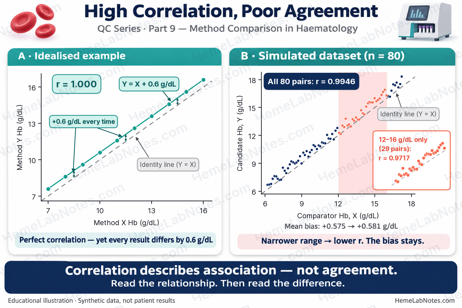
Figure 1. Correlation under a fixed offset and range restriction.
View full size3. Design the Comparison Before Collecting Results
CLSI EP09c addresses measurement-procedure comparison and bias estimation using patient samples. ICSH and CLSI H26 provide haematology-specific guidance for analyser evaluation, verification and quality assurance [1,2,6]. The study size and design must follow the specific claim: a full system evaluation, verification of a second instrument, and investigation of bias at one clinical decision point do not automatically require identical designs.
- Define the claim. Is the new analyser intended to replace the old one, operate interchangeably, or support only a defined subset of testing?
- Choose the comparator carefully. An established routine analyser is a practical comparator, but is not automatically a reference measurement procedure or analytical truth. If its imprecision is relevant, it must be accounted for.
- Set acceptance criteria in advance. Specify allowable systematic bias, individual-result agreement if interchangeability matters, decision-point requirements, and any separate imprecision requirements. Base them on a defensible clinical or analytical performance specification [1,7].
- Cover relevant concentrations. Include specimens across the intended reportable interval and deliberately represent abnormal values and clinical decision points. An overall Hb study with only a handful of samples near 7 g/dL gives limited evidence about that threshold.
- Control specimen handling. Define timing, sample stability, mixing, order of testing, handling of flagged samples, and how delays will be prevented from creating misleading differences.
- Document QC and precision. Check that both analysers are operating acceptably. A paired-method study does not independently establish within-run precision or full analytical performance [1,2,6].
- Investigate discrepant pairs. Record clots, platelet clumping, cold agglutinins, instrument flags and other potential interferences. Prespecify exclusions; do not silently discard inconvenient data.
The sample counts described in guidance for a full analyser evaluation must not be presented as universal requirements for every local verification [2].
4. Start With Plots, Not a Single Statistic
Scatter plot: Y against X
Plot the candidate (Y) against the designated comparator (X). Include the identity line (Y = X) as well as any fitted regression line. The identity line represents exact agreement; a good regression fit does not.
Look for curvature, outliers, isolated groups, changing scatter, and gaps near clinically important concentrations. If the two methods disagree systematically, a regression line can look very convincing while running above the identity line.
Difference plot: choose the horizontal axis deliberately
For each paired sample, calculate the signed difference:
dᵢ = Yᵢ − Xᵢ
Positive values mean that the candidate reports higher. A conventional Bland–Altman plot places the pair mean, mᵢ = (Xᵢ + Yᵢ)/2, on the horizontal axis. This avoids some misleading mathematical coupling that can arise when differences are plotted against an imprecise comparator [4,5,8].
There is an important qualification. Plotting Y − X against X is defensible when X is a reference method, or demonstrably much more precise than Y, because X can then serve as a reasonable estimate of the underlying measurand. Krouwer has argued for this reference-method use [9]. If both routine analysers have similar imprecision, the error in X appears in both axes and can generate an artifactual trend even when no true concentration-dependent bias exists [8]. A pair-mean plot is ordinarily more suitable for assessing two similarly imperfect methods; it is not immune to all artefacts if their variances differ substantially [5,8,9].
For this article’s synthetic data only, the designated comparator X is treated as error-free after its displayed rounding; all generated random measurement error is assigned to Y. Thus difference-versus-X is reasonable for this controlled simulation. Real analyser comparisons rarely satisfy this assumption. Their relative imprecision should guide the plot, regression, and interpretation.
A difference plot helps investigate bias; a Bland–Altman analysis of differences adds estimates of the mean and individual-result spread. Neither choice of horizontal axis independently resolves a poor study design.
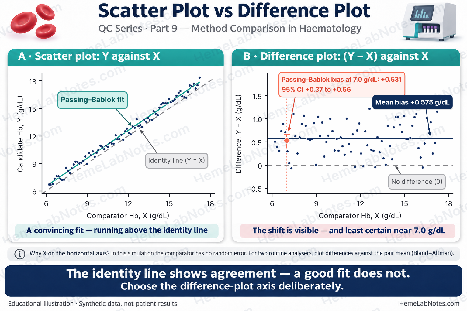
Figure 2. Scatter and difference-versus-X for the fixed-X teaching simulation.
View full size5. What Regression Can — and Cannot — Tell Us
A common method-comparison relationship is written:
Y = a + bX
Here a is the intercept and b is the slope. If a linear model is appropriate, an intercept different from zero can suggest a constant component of bias; a slope different from one can suggest a proportional component. Because intercepts are often extrapolated far outside the observed concentration range, estimated bias at a relevant concentration is usually the more useful quantity:
Estimated bias at X₀ = (a + bX₀) − X₀ = a + (b − 1)X₀.
Selecting regression appropriately
- Passing–Bablok regression is a robust, nonparametric linear procedure. It assumes that a linear relationship is appropriate and needs suitable measurement ranges and sufficiently continuous quantitative data. Its robustness does not excuse nonlinearity, a narrow range, or inadequate coverage of clinical decision points [3].
- Deming regression accounts for measurement error in both X and Y but needs the relative error-variance ratio to be justified; choosing a ratio of 1 without precision evidence is not automatically appropriate [1]. Weighted options may be needed if error variance changes with concentration.
- Ordinary least squares (OLS) treats X as known without relevant measurement error. That assumption is inappropriate for many real two-analyser comparisons. It is, however, consistent with the conditional model used to create our synthetic example, in which X was fixed and random noise was added only to Y.
Different regression approaches can return similar estimates when the measurement range is broad and correlation is high. This agreement alone does not justify a method choice; methods can diverge substantially in other datasets or under different error structures.
A confidence interval for the slope that includes 1 means that a proportional departure was not established at that confidence level. It does not demonstrate an absence of proportional bias. Likewise, a fitted line that does not differ significantly from identity is not proof of clinical equivalence. A proposed acceptance decision needs a prespecified tolerance and its uncertainty, especially at relevant decision points [1,3].
6. Bland–Altman Analysis: How Far Apart Are Individual Results?
For n independent paired samples, define:
- dᵢ = Yᵢ − Xᵢ, the signed paired difference.
- mᵢ = (Yᵢ + Xᵢ)/2, the paired mean.
- Mean bias, d̄ = Σdᵢ/n.
- SDd, the sample standard deviation of differences using denominator n − 1.
If the differences are approximately normal and have reasonably stable mean and variance across the relevant range, the customary 95% limits of agreement (LoA) are:
Lower LoA = d̄ − 1.96 × SDd
Upper LoA = d̄ + 1.96 × SDd
These estimate the spread expected to contain approximately 95% of individual differences under the model. They are not an acceptance band and should not be interpreted as guaranteeing that two methods are interchangeable [4,5].
Do the assumptions hold?
Inspect differences for nonlinearity, outliers, concentration-dependent bias, and heteroscedasticity. Fixed LoA can be misleading if the mean or SD of differences varies substantially with concentration. Consider suitable transformations (including ratios or percentages where defensible), stratified assessment, or regression-based limits [5]. Near zero, percentage differences can be unstable and need particular care.
Formal tests may help describe the data but should not replace graphical and clinical review. A non-significant normality, trend, or heteroscedasticity test is not proof that the corresponding issue is absent. A small or poorly distributed study can lack power to detect meaningful problems.
Mean bias CI versus LoA CI
The 95% confidence interval (CI) of mean bias quantifies uncertainty in an estimate of the average difference. With n pairs, the usual t-based interval is:
95% CI for mean bias = d̄ ± t₀.₉₇₅,ₙ₋₁ × SDd/√n.
By contrast, the LoA describe individual-result differences, and the estimates of each LoA also have uncertainty. One illustrative large-sample normal-theory approximation is:
SE(LoA) ≈ SDd × √[1/n + 1.96²/{2(n − 1)}]
Approximate 95% CI for each LoA = estimated LoA ± t₀.₉₇₅,ₙ₋₁ × SE(LoA).
These are approximate intervals; other established CI approaches can yield slightly different endpoints. An apparently precise LoA point estimate can still have a clinically important margin of uncertainty [5].
7. Worked Example — A High Correlation With Individual Differences That Fail a Hypothetical Criterion
This teaching dataset contains 80 independently simulated Hb pairs, with comparator X from 6.20 to 17.20 g/dL. The designated comparator was generated as a fixed, rounded linear series, while the candidate was generated by adding a fixed offset and random noise to the already rounded X. Thus the simulation assumes error-free X (apart from displayed-value quantisation) and random error in Y only. This is not a realistic universal model of two routine analysers.
Reproducible summary
| Statistic | Result from 80-pair CSV |
|---|---|
| Pearson correlation, r | 0.9946 |
| Mean bias, Y − X | +0.5754 g/dL |
| SDd | 0.3425 g/dL |
| 95% LoA | −0.0960 to +1.2468 g/dL |
| t-based 95% CI of mean bias (t₇₉ = 1.990) | +0.4991 to +0.6516 g/dL |
| Approximate 95% CI for lower LoA | −0.2268 to +0.0348 g/dL |
| Approximate 95% CI for upper LoA | +1.1159 to +1.3776 g/dL |
The high r reflects a strong linear relationship. But the candidate is, on average, 0.575 g/dL higher, and individual paired differences are much more variable than the average alone suggests.
Regression on the same pairs
Using a conventional Passing–Bablok slope-ranking implementation (including the original handling of slopes below −1) gives approximately:
| Regression result | Synthetic estimate |
|---|---|
| Passing–Bablok slope | 1.012 (approximate 95% CI 0.987–1.038) |
| Passing–Bablok intercept | +0.445 g/dL (approximate 95% CI +0.169 to +0.717) |
| Estimated bias at X = 7.0 g/dL | +0.531 g/dL |
| Passing–Bablok bootstrap 95% CI for bias at 7.0 g/dL | +0.37 to +0.66 g/dL |
| OLS slope / intercept | 1.009 / +0.473 g/dL |
| OLS estimated bias at 7.0 g/dL (t-based 95% CI) | +0.534 g/dL (+0.399 to +0.669) |
| Illustrative unweighted Deming slope / intercept, error-variance ratio 1 | 1.014 / +0.407 g/dL |
The Passing–Bablok slope CI includes 1, whereas the intercept CI excludes 0. This supports a predominantly positive constant component of bias, without statistically established proportional bias in this dataset. It does not prove that proportional bias is exactly zero. Confidence intervals, especially for an intercept, are implementation-dependent; ties from rounding and the treatment of slopes equal to −1 can change the last reported digits. Because X is treated as error-free in this simulation, OLS matches its generating assumptions; the Deming ratio-of-1 calculation is supplied only as a numerical contrast and does not match the simulation’s error structure.
Both uncertainty intervals at 7.0 g/dL were calculated from these same 80 pairs. For OLS, the interval is a t-based 95% confidence interval for the fitted mean response at X = 7.0 g/dL, with X treated as fixed and error-free; it is not a prediction interval for one new measurement. For Passing–Bablok, the percentile 95% CI was obtained by resampling complete (X, Y) pairs 2,000 times with replacement (seed 1) and recalculating the estimated bias. Bootstrap estimates depend on the resampling design and implementation, particularly when the target is near the boundary of the sampled range. Bootstrap limits vary by about ±0.01–0.02 g/dL with a different seed for this 2,000-resample teaching example, so the reported limits are rounded to two decimal places.
The OLS decision-point CI has a half-width of approximately 0.135 g/dL; the slightly asymmetric Passing–Bablok bootstrap interval extends approximately 0.16 g/dL below and 0.13 g/dL above its point estimate. Both are markedly wider than the approximately 0.076 g/dL half-width of the overall mean-bias CI. Only six comparator readings are below 7.0 g/dL, so this threshold lies near the lower edge of the study’s coverage. The clinically important point may be where the data are least informative. A dedicated decision-point study would require more representative samples; neither interval alone demonstrates clinical acceptability.
For clinical decisions, focus on the estimated bias and its uncertainty at the relevant concentration, not on the significance of a slope/intercept considered in isolation. This small teaching study cannot establish interchangeability near a decision threshold.
A hypothetical ±0.5 g/dL individual-pair band
Suppose the laboratory has prospectively specified that each paired result should differ by no more than ±0.5 g/dL across the selected Hb range. For this particular hypothetical criterion, a pair is counted as outside only if:
|dᵢ| > 0.5 g/dL, not |dᵢ| ≥ 0.5 g/dL.
Accordingly, 47/80 (58.8%) are outside the band, all on the positive side. Pair S026 has d = +0.50 g/dL and is inside under this inclusive-boundary rule. The ±0.5 band is not an EP09c, CLSI, ICSH or universal Hb limit.
A specific pair, S006, is 6.90 g/dL on X and 7.61 g/dL on Y. Of the six pairs with comparator X < 7.0 g/dL, three (S004, S005, S006) have candidate Y > 7.0 g/dL. Of the 13 pairs with comparator X < 8.0 g/dL, three (S010, S011, S013) have candidate Y > 8.0 g/dL. All six threshold crossings in these two counts are upward; none is downward. A positive shift may make an Hb result appear less low, a direction of concern when assessing severe anaemia. These are illustrations of crossing numerical thresholds, not a measured rate of inappropriate transfusion decisions. Clinical decisions depend on the patient’s condition and applicable guidance, not a single Hb number.
The Passing–Bablok estimated bias at 7.0 g/dL is +0.531 g/dL (7.6%). At 14.0 g/dL, the same fitted line implies +0.618 g/dL (4.4%). A primarily absolute/constant bias can therefore have a larger percentage effect in the low-Hb range. Compare any such result against the laboratory’s own defensible, prespecified performance specifications for the clinical application [7]; the percentages here are not universal acceptance limits.
Does correcting average bias fix agreement?
The 47 pairs outside ±0.5 g/dL all have positive differences. The average positive shift is therefore an important contributor: the mean bias (+0.5754 g/dL) itself exceeds the hypothetical +0.5 boundary.
Now make a purely arithmetic counterfactual: subtract the observed mean bias from every Y, then recompute the absolute residual differences. The centred mean difference becomes zero, but 12/80 pairs still have |dᵢ − d̄| > 0.5 g/dL. The SDd is unchanged, and the model’s 95% LoA half-width remains approximately ±0.671 g/dL.
This illustrates a practical distinction: removing an average offset does not remove dispersion among individual results. It is not a claim that physically recalibrating an analyser would necessarily produce this result; real recalibration can alter error behaviour and would require a fresh evaluation. From a paired study alone, that remaining spread also cannot be assigned to one specific analyser without further precision evidence.
Use precision to investigate the spread. If the two analysers’ random errors are independent, their repeatability SDs are relevant at the same Hb concentration, and sample handling adds negligible variation, the expected SD of pairwise differences is approximately √(SDₓ² + SDᵧ²). An observed SDd substantially larger than this expectation merits investigation for stability, interference, timing or other sources of additional variation. Those assumptions must be checked: repeated measurements, possible covariance and concentration-dependent imprecision can change the calculation. In this one-error-source simulation, the input noise SD was 0.30 g/dL, while the observed SDd is 0.343 g/dL (normal-theory, chi-square 95% CI: 0.296–0.406 g/dL, assuming independent approximately normal differences). This range includes 0.30; it is compatible with the generating noise, not proof that the real-world imprecision model has been verified. The paired-sample SDd is not a substitute for a dedicated precision study [6].
Assumption checks, not assumption proofs
On these 80 differences:
- Shapiro–Wilk normality test: p = 0.059.
- Pearson correlation of difference with X (appropriate to this simulation’s fixed, error-free X): r = 0.083, p = 0.464.
- Pearson correlation of difference with paired mean (the conventional Bland–Altman display axis): r = 0.135, p = 0.232.
- Spearman correlation of absolute centred residual |dᵢ − d̄| with paired mean: ρ = 0.130, p = 0.249.
No strong violation is apparent from these checks in the teaching dataset, but none establishes normality, absence of concentration-dependent bias, or homoscedasticity. Even with error-free X, plotting d against the pair mean introduces a small positive mathematical coupling because Y contributes to both quantities; the d-versus-X check is therefore more directly interpretable for this simulation. The plotted data remain essential, as does a concentration range with sufficient clinically relevant representation.
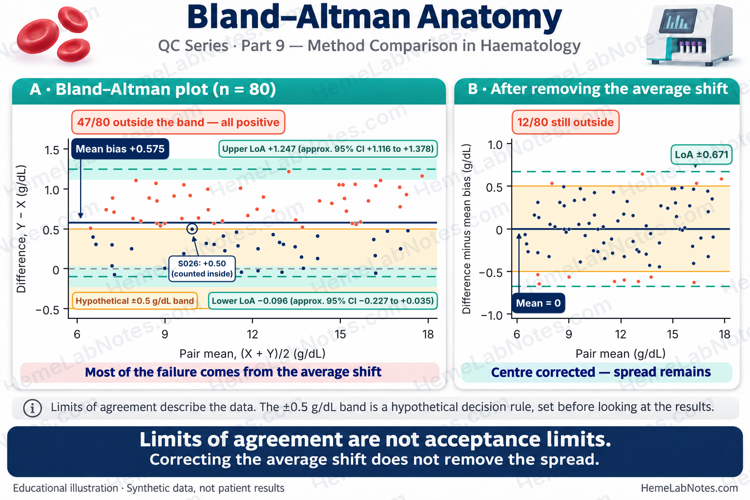
Figure 3. Bland–Altman and arithmetic mean-centering.
View full size8. Haematology-Specific Questions Worth Asking
One global correlation result can hide quite different performance across a complete blood count. Each clinically important measurand and interval deserves its own evaluation.
- Haemoglobin: Is systematic bias acceptable at low Hb concentrations? Are the errors large enough to affect local reporting, delta checks, or clinical assessment?
- Platelets: Does agreement hold in thrombocytopenic specimens, rather than only across normal counts? Investigate platelet clumping, giant platelets, and counting-principle differences where relevant.
- WBC: Have low WBC counts and markedly raised counts been represented? Are flags, abnormal cell populations and sample-related interferences changing comparability?
- RBC and calculated indices: Are differences in MCV, RBC, Hb and Hct internally plausible? Could cold agglutination or another specimen-specific problem be contributing?
A reassuring relationship for normal Hb does not establish agreement for PLT at transfusion-related thresholds, or for abnormal WBC flags. Investigate clinically discordant samples, not just the aggregate regression result [2,6].
9. A Bench-First Decision Workflow
- Validate the experiment. Check specimen quality, analysis timing, mixing, QC, selection and exclusion rules, and concentration coverage.
- Inspect plots. Compare scatter against the identity line; choose a defensible difference-plot horizontal axis and inspect for outliers, trends and heteroscedasticity.
- Estimate systematic bias. Use a regression model consistent with the error structure and estimate bias around important clinical decision points with uncertainty.
- Assess individual-result spread. Where assumptions permit, calculate signed differences, LoA, and confidence intervals for the LoA; investigate concentration-dependent patterns when a fixed LoA model fails.
- Use prespecified acceptance limits. Keep tolerances for systematic bias, individual differences and imprecision conceptually separate. Do not replace these with an r cutoff or a non-significant regression test.
- Determine what the failure represents. A positive mean shift may have a correctable systematic cause, but shifting results does not automatically reduce pairwise variation. Compare observed SDd with the spread expected from independent precision estimates, where justified: SDd,expected ≈ √(SDₓ² + SDᵧ²). Consider instability or specimen-specific interference when the observed spread is unexpectedly large. Investigate both centre and spread, then revalidate after an intervention. The arithmetic correction in Section 7 is illustrative, not a validated calibration procedure.
- Document a scoped decision. State which measurands, concentration ranges and clinical applications have evidence of adequate performance, and which do not. A method-comparison study is one component of analyser validation, not the entire process.
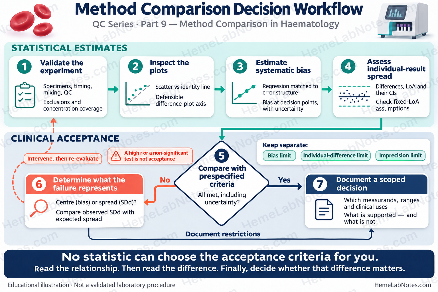
Figure 4. Method comparison decision workflow separating statistical estimates from clinical acceptance.
View full size10. The Take-Home Message
Correlation says that two analysers move together. Regression helps describe systematic relationships and estimate bias at particular concentrations. Bland–Altman analysis helps show how far apart individual paired results may be.
None of these statistics can choose the laboratory’s acceptance criteria for it. That decision depends on the intended clinical use, suitable study coverage, justified performance specifications, and the uncertainty in the results.
Read the relationship. Then read the difference. Finally, decide whether that difference matters.
Reproducibility Note — Educational Dataset
Source of truth:
QC09_Synthetic_Hb_Method_Comparison_V0.1.1.csv(80 fixed synthetic pairs). The CSV, not any random-number seed, defines the published teaching dataset. Comparator X, candidate Y and signed differences are displayed to two decimal places; the pair mean is retained to three decimals, calculated from the displayed X and Y values. No actual patient or manufacturer dataset is used.For environment-dependent regeneration, the verified Python construction is
X = np.round(np.linspace(6.2, 17.2, 80), 2)followed byrng = np.random.Generator(np.random.PCG64(20261105))andY = np.round(X + 0.55 + rng.normal(0, 0.30, size=80), 2). Add noise after rounding X. Recalculate differences and pair means from the rounded X and Y. NumPy’s randomGeneratordoes not guarantee identical streams across all versions and environments, even when PCG64 and the seed are explicit; compare any reconstruction with the authoritative CSV rather than assuming portability.Statistical implementation: Passing–Bablok slopes and their rank-based interval are calculated from pairwise slopes after the documented exclusion of −1 slopes, with the appropriate rank shift. The corrected lower 0-based slope-CI index is
M1 + K - 1, whereM1 = round((N − C)/2)is derived from a 1-based rank convention; the upper 0-based index isN − M1 + K. With these data the corrected index points to a tied value, so the displayed lower CI stays 0.987. Decision-point Passing–Bablok CI uses the 2.5th and 97.5th percentile of 2,000 complete-pair bootstrap replicates (seed 1) at 7.0 g/dL. OLS CI uses a t-based uncertainty interval for the fitted mean at that X, not a prediction interval. These are transparent teaching implementations, not a validated clinical statistics tool or a reproduction of CLSI proprietary tables.
References
- Clinical and Laboratory Standards Institute (CLSI). Measurement Procedure Comparison and Bias Estimation Using Patient Samples. 3rd ed. CLSI guideline EP09c. Wayne, PA: CLSI; 2018. https://clsi.org/shop/standards/ep09/
- International Council for Standardization in Haematology, Writing Group; Briggs C, Culp N, Davis B, d’Onofrio G, Zini G, Machin SJ. ICSH guidelines for the evaluation of blood cell analysers including those used for differential leucocyte and reticulocyte counting. Int J Lab Hematol. 2014;36(6):613–627. https://doi.org/10.1111/ijlh.12201
- Passing H, Bablok W. A new biometrical procedure for testing the equality of measurements from two different analytical methods. Application of linear regression procedures for method comparison studies in clinical chemistry, Part I. J Clin Chem Clin Biochem. 1983;21(11):709–720. https://doi.org/10.1515/cclm.1983.21.11.709
- Bland JM, Altman DG. Statistical methods for assessing agreement between two methods of clinical measurement. Lancet. 1986;1(8476):307–310. https://pubmed.ncbi.nlm.nih.gov/2868172/
- Bland JM, Altman DG. Measuring agreement in method comparison studies. Stat Methods Med Res. 1999;8(2):135–160. https://doi.org/10.1177/096228029900800204
- Clinical and Laboratory Standards Institute (CLSI). Validation, Verification, and Quality Assurance of Automated Hematology Analyzers. 2nd ed. CLSI document H26-A2. Wayne, PA: CLSI; 2010 (reaffirmed September 2016). https://clsi.org/shop/standards/h26/
- Sandberg S, Fraser CG, Horvath AR, Jansen R, Jones G, Oosterhuis W, et al. Defining analytical performance specifications: Consensus Statement from the 1st Strategic Conference of the European Federation of Clinical Chemistry and Laboratory Medicine. Clin Chem Lab Med. 2015;53(6):833–835. https://doi.org/10.1515/cclm-2015-0067
- Bland JM, Altman DG. Comparing methods of measurement: why plotting difference against standard method is misleading. Lancet. 1995;346(8982):1085–1087. https://doi.org/10.1016/S0140-6736(95)91748-9
- Krouwer JS. Why Bland–Altman plots should use X, not (Y + X)/2 when X is a reference method. Stat Med. 2008;27(5):778–780. https://doi.org/10.1002/sim.3086