The morning QC has passed.
All three control levels are acceptable, and the analyser is ready for patient samples.
But this time, instead of looking only at PASS or FAIL, I open the QC summary.
For each parameter, the analyser displays a Mean, Standard Deviation (SD) and Coefficient of Variation (CV).
These numbers are familiar. We see them in QC reports, precision studies and instrument performance summaries.
But how often do we stop to consider what they actually mean?
A low CV looks reassuring. A small SD suggests good precision. A mean close to the expected target appears acceptable.
Yet none of these statistics tells the complete story on its own.
To understand QC properly, we need to understand what each statistic describes — and how the three work together.
1. The Mean: Where Are Our QC Results Centred?
The mean is the average of a group of measurements.
It provides a central value around which repeated QC results may be distributed.
We calculate it by adding all the results and dividing by the number of measurements.
Mean = Sum of all measurements ÷ Number of measurements
Consider six HGB control results obtained from the same control level.
These are the same measurements introduced in QC Article 01 when we discussed the difference between precision and accuracy.
| Run | HGB (g/dL) |
|---|---|
| 1 | 12.3 |
| 2 | 12.4 |
| 3 | 12.4 |
| 4 | 12.5 |
| 5 | 12.4 |
| 6 | 12.4 |
The mean is:
Mean = (12.3 + 12.4 + 12.4 + 12.5 + 12.4 + 12.4) ÷ 6
Mean = 12.40 g/dL
This tells us where the six measurements are centred.
But there is something important the mean cannot tell us.
A mean close to the expected target does not necessarily mean the measurement procedure is precise.
Two sets of results — the same mean, different variation
Now consider another set of six HGB measurements.
| Run | Dataset A (g/dL) | Dataset B (g/dL) |
|---|---|---|
| 1 | 12.3 | 12.0 |
| 2 | 12.4 | 12.8 |
| 3 | 12.4 | 12.2 |
| 4 | 12.5 | 12.6 |
| 5 | 12.4 | 12.4 |
| 6 | 12.4 | 12.4 |
| Mean | 12.40 | 12.40 |
Both sets have exactly the same mean.
But Dataset A is tightly grouped around 12.40 g/dL, while Dataset B varies much more widely.
We will see how SD and CV are calculated in the next two sections.
Using the sample SD calculation, their statistical summaries are:
| Statistic | Dataset A | Dataset B |
|---|---|---|
| Mean | 12.40 g/dL | 12.40 g/dL |
| SD | 0.0632 g/dL | 0.2828 g/dL |
| CV | 0.51% | 2.28% |
The average alone cannot reveal this difference.
If we looked only at the mean, we might mistakenly think both sets demonstrated similar measurement performance.
This is why we need another statistic.
2. Standard Deviation: How Much Do the Results Vary?
Standard Deviation (SD) describes how widely measurements are distributed around their mean.
For routine QC calculations using a sample of observed results, the sample SD is commonly calculated as:
Sample SD = √[Σ(xᵢ − Mean)² ÷ (n − 1)]
Where:
- SD = sample standard deviation
- Σ = sum of the indicated values
- xᵢ = each individual measurement
- Mean = average of the measurements
- n = number of measurements
Let’s use Dataset A from the previous section.
We already know the mean is 12.40 g/dL.
Step 1 — Calculate each difference from the mean
| HGB | Difference from mean | Squared difference |
|---|---|---|
| 12.3 | −0.1 | 0.01 |
| 12.4 | 0.0 | 0.00 |
| 12.4 | 0.0 | 0.00 |
| 12.5 | +0.1 | 0.01 |
| 12.4 | 0.0 | 0.00 |
| 12.4 | 0.0 | 0.00 |
| Total | 0.02 |
Step 2 — Divide by n − 1
There are six measurements, so the denominator is five.
Sample variance = 0.02 ÷ 5
Sample variance = 0.004 (g/dL)²
Step 3 — Calculate the square root
SD = √0.004
SD = 0.0632 g/dL
Rounded to two decimal places, the SD is approximately 0.06 g/dL.
The results are tightly grouped around their mean.
That is evidence of good repeatability within this small illustrative dataset.
Now compare this with Dataset B.
Its sum of squared deviations is 0.40.
Sample variance = 0.40 ÷ 5 = 0.08
SD = √0.08
SD = 0.2828 g/dL
The contrast is clear.
Dataset B has the same mean as Dataset A but approximately 4.5 times the sample SD.
However, six measurements are not sufficient to establish reliable long-term laboratory QC limits.
They demonstrate the calculation, not the complete analytical performance of the analyser.
What does a larger SD mean?
For measurements at the same concentration, using comparable conditions and an appropriate statistical model, a larger SD generally indicates greater variation.
A smaller SD indicates tighter grouping of measurements.
This is closely related to analytical precision.
But be careful.
SD describes variation in the observed data. It does not, by itself, establish that the results are accurate. [1,2]
An analyser may repeatedly produce almost identical results while consistently measuring above or below a reliable reference value.
The results are precise, but systematic bias may still be present.
3. Coefficient of Variation: Why Express SD as a Percentage?
SD is expressed in the same measurement units as the parameter being analysed.
For HGB, the SD is expressed in g/dL.
For MCV, it is expressed in fL.
For WBC and PLT, it may be expressed in ×10⁹/L.
This makes direct comparisons between different measurements difficult.
The Coefficient of Variation (CV) expresses SD relative to the mean, as a percentage.
CV (%) = SD ÷ Mean × 100
Using Dataset A:
CV = 0.0632 ÷ 12.40 × 100
CV = 0.51%
For Dataset B:
CV = 0.2828 ÷ 12.40 × 100
CV = 2.28%
Both datasets have the same mean.
But Dataset B has a much higher CV because its measurements vary more widely.
This provides a convenient way to describe relative analytical variation.
But does a lower CV always mean the result is clinically more reliable?
Not necessarily.
A haematology example: platelet QC
Consider two illustrative platelet control levels.
| Parameter | Low PLT QC | Normal PLT QC |
|---|---|---|
| Mean (×10⁹/L) | 40 | 250 |
| SD (×10⁹/L) | 3 | 5 |
| CV | 7.5% | 2.0% |
The normal-level control has a larger absolute SD but a smaller relative CV.
The low-level control has a smaller absolute SD but a higher CV.
Neither statistic is incorrect.
They describe different aspects of variation.
At low platelet concentrations, the same absolute difference can represent a much larger percentage of the measured value.
This becomes important when the laboratory is assessing performance near clinically relevant decision points.
For example, variation around a severely thrombocytopenic platelet concentration may have different implications from similar variation at a normal platelet concentration.
Therefore, the question should not simply be:
“Which CV is lower?”
A more useful question is:
“Is the observed imprecision acceptable at the concentration where clinical decisions are made?”
This requires an appropriate analytical performance specification and an understanding of the intended clinical use.
The numbers in this example are illustrative; they are not universal acceptance criteria for platelet QC.
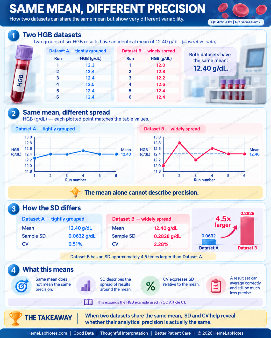
Figure 1. Two HGB datasets can have the same mean but very different variation. Sample SD and CV help describe their relative precision.
View full size4. Understanding Normal Analytical Variation
Even a stable analytical system does not produce exactly the same result every time.
Small fluctuations occur because measurement procedures are subject to random analytical variation.
For many quantitative QC measurements, the distribution of results can be approximated by a normal or Gaussian distribution.
Under that assumption, we expect approximately:
| Range around the mean | Expected proportion |
|---|---|
| Mean ±1 SD | 68.3% |
| Mean ±2 SD | 95.5% |
| Mean ±3 SD | 99.7% |
These percentages assume a stable process and an approximately normal distribution.
They are not universal guarantees for every parameter, control material or analyser.
What do these limits look like?
Consider a separate, illustrative HGB control with an established:
Mean = 12.40 g/dL
SD = 0.08 g/dL
The SD of 0.08 g/dL is slightly larger than the approximately 0.06 g/dL obtained from Dataset A’s six consecutive measurements.
This is consistent with the possibility that a longer monitoring period captures additional sources of analytical variation.
However, a longer-period SD is not necessarily larger in every situation. The result depends on the study design, data quality and stability of the measurement process.
For this illustration, the statistical limits are:
| Control boundary | HGB (g/dL) |
|---|---|
| +3 SD | 12.64 |
| +2 SD | 12.56 |
| +1 SD | 12.48 |
| Mean | 12.40 |
| −1 SD | 12.32 |
| −2 SD | 12.24 |
| −3 SD | 12.16 |
These are statistical boundaries calculated from the illustrative mean and SD, not automatically approved laboratory control limits.
Now imagine today’s HGB QC result is 12.53 g/dL.
It is higher than the mean, but still below +2 SD.
How far from the mean is it?
We can express the difference as an SD score:
SD score (z) = (Observed result − Mean) ÷ SD
z = (12.53 − 12.40) ÷ 0.08
z = 0.13 ÷ 0.08
z = +1.625 ≈ +1.63 SD
The result is approximately +1.63 SD above the mean.
That tells us its relative position within the expected QC distribution.
It does not automatically tell us whether the analytical run should be accepted or rejected.
That decision depends on the laboratory’s selected QC rules, the other control results and recent QC history. [1,3]
Being within ±2 SD is not, by itself, proof that the entire QC run has passed.
Consecutive results, multi-level patterns and other statistical decision rules may identify a problem even when individual results remain within simple limits.
This distinction becomes especially important when interpreting Levey–Jennings charts.
5. Which SD Are We Actually Using?
This is one of the most easily overlooked questions in QC.
An SD calculated from six consecutive measurements does not necessarily represent the same sources of variation as an SD calculated from daily QC results collected over several weeks.
The first may mainly reflect short-term repeatability.
The second may include variation occurring across different days, analytical runs, operators or routine operating conditions.
These are not interchangeable measurements of precision.
Consider three situations:
| Situation | What the data mainly describe |
|---|---|
| Six repeated measurements in one run | Short-term repeatability |
| Repeated measurements across multiple days and runs | A broader component of within-laboratory precision |
| Routine QC results collected over a representative stable period | Variation observed under the laboratory’s QC monitoring conditions |
CLSI EP15 describes structured laboratory procedures for verifying precision claims and estimating bias. Such verification studies have defined designs and analytical objectives; they should not be confused with simply calculating CV from a handful of routine QC measurements. [4]
For daily QC monitoring, the laboratory needs an appropriately established mean and SD that reflect a stable measurement procedure under relevant routine conditions.
CLSI C24 provides guidance on selecting QC strategies and establishing appropriate target values and SDs for control materials. [1]
Why the data collection period matters
Suppose we run the same HGB control six times within a few minutes.
The results are remarkably similar.
The CV is very low.
That is reassuring for short-term repeatability.
But it does not demonstrate that the analyser will maintain the same performance throughout the next month.
Additional variation may appear between runs, across days, after maintenance or under other routine operating conditions.
A meaningful QC baseline must therefore be established using a suitable amount of representative, stable data according to the laboratory’s procedure.
A low short-term CV should not automatically be used to set long-term QC acceptance limits.
What if the QC system is already changing?
There is another problem.
Imagine calculating a new SD from a period during which the analytical system is gradually drifting.
The increased spread may produce a larger calculated SD.
If we then use that inflated SD to establish new control limits without investigating the underlying change, the limits may become less sensitive to important analytical problems.
The same issue can occur when an unexplained shift is incorporated into a revised mean.
Do not redefine the expected QC performance simply to accommodate unexplained analytical changes.
The laboratory should first determine whether the process was stable and whether the data are appropriate for establishing or revising QC limits.
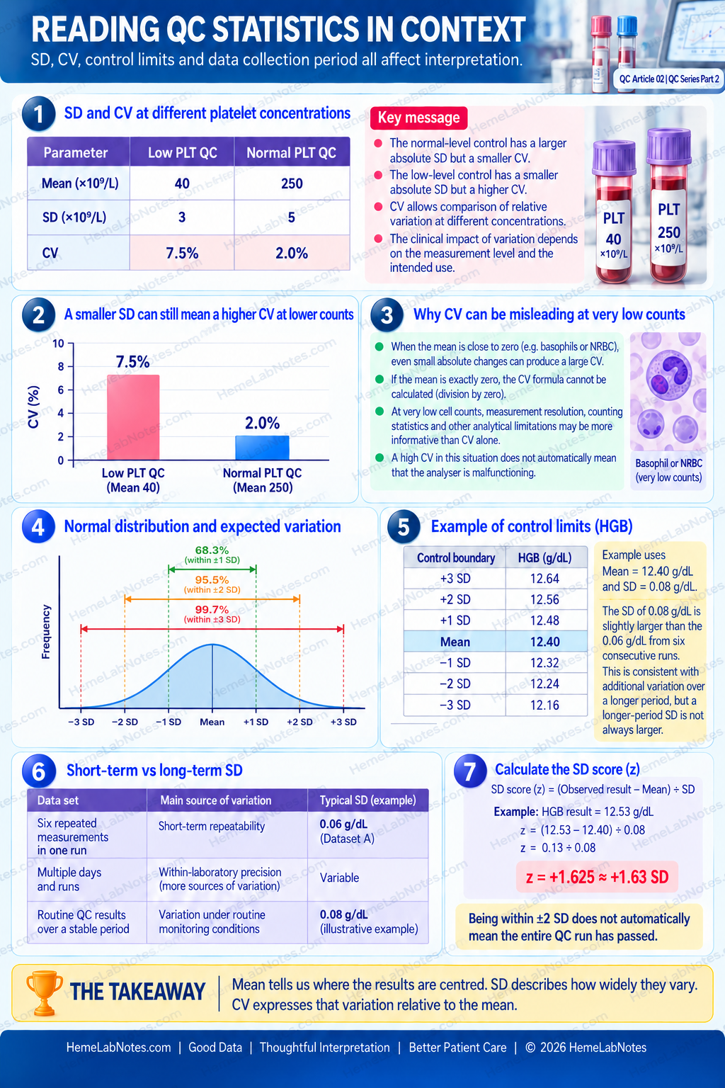
Figure 2. Mean, SD and CV must be interpreted in the context of concentration, analytical conditions, data collection period and laboratory QC rules.
View full size6. Reading Mean, SD and CV Together
When I review a QC summary, I do not want to judge analytical performance from a single statistic.
I prefer to understand how the mean, SD and CV relate to one another.
Consider these illustrative situations:
| Observation | Possible interpretation |
|---|---|
| Mean stable, SD and CV stable | Consistent with stable performance under monitored conditions |
| Mean changes, SD remains similar | Possible systematic change requiring investigation |
| Mean similar, SD increases | Increased variability or imprecision may be present |
| CV rises at a low concentration | Relative imprecision may be increasing; examine the absolute SD and concentration |
| Mean and SD both change | Could reflect several causes; review the underlying QC data and events |
These patterns are clues, not diagnoses.
For example, an increasing SD does not automatically prove an instrument malfunction.
The change might involve the control material, its handling, measurement conditions or the measurement procedure itself.
Likewise, a change in the mean may reflect a reagent or calibration change, a new QC target assignment, a control-material effect or another analytical change.
The correct response is to investigate the evidence and its context.
The numbers tell us what has changed statistically.
They do not necessarily tell us why.
A final caution about CV
CV is particularly useful for comparing relative imprecision at different concentrations.
However, a CV percentage should not be interpreted independently of the measurement level, observed SD and relevant analytical performance specifications.
For measurements whose mean approaches zero, CV can also become unstable or inappropriate.
Consider an absolute basophil count or NRBC count that is very close to zero.
Even small absolute changes may generate a large CV because the mean is so small.
If the mean is exactly zero, the CV formula involves division by zero and cannot be calculated.
At very low cell counts, the measurement’s resolution, counting statistics and other analytical limitations may be more informative than CV alone.
A high CV in this situation does not automatically mean that the analyser is malfunctioning.
In practical haematology, the important question is whether the observed variation is acceptable for the parameter and the concentrations at which decisions are made.
That is more meaningful than treating the lowest CV as automatically the best result.
7. Beyond the Statistics: What Should We Look at Next?
Mean, SD and CV provide the statistical foundation of daily QC.
But they are still summaries.
They do not show the sequence in which individual results occurred.
Two sets of QC measurements can have similar means and SDs while displaying very different patterns over time.
One may fluctuate randomly around the target mean.
Another may show a sustained change or an emerging directional pattern.
If we only examine the summary statistics, we may miss the timing and behaviour of those changes.
This is where the Levey–Jennings chart becomes valuable.
By plotting QC measurements in sequence against an established mean and SD, we can begin to recognise patterns that warrant further investigation.
The chart also allows laboratories to apply their selected statistical QC rules.
An apparently unusual sequence should be evaluated using the laboratory’s defined rules rather than automatically labelled as a shift, trend or drift.
Those distinctions will become important in later articles.
For now, the principle is straightforward:
Mean tells us where the results are centred. SD tells us how widely they vary. CV tells us how large that variation is relative to the mean.
Understanding all three gives us a stronger foundation for evaluating analytical performance.
The Takeaway
Mean, SD and CV are more than numbers displayed in a QC summary.
They describe different characteristics of analytical data.
The mean identifies the central value.
SD describes the spread of the measurements.
CV expresses that variation relative to the mean.
But none of them proves that every patient result is accurate or that the measurement system is free from error.
Their usefulness depends on how the data were collected, whether the analytical process was stable, and which clinical and analytical performance requirements apply.
A good QC review therefore goes beyond asking whether the CV is low or the mean is close to target.
It asks whether the observed performance is consistent, appropriate and sufficiently reliable for the measurements we report.
The statistics describe the variation. The laboratory must decide whether that variation is acceptable.
Coming Next — QC Series Part 3
Reading the Levey–Jennings Chart: When QC Starts Telling a Story
How do individual QC results behave over time?
Why can several apparently acceptable QC values still indicate a problem?
And how should we interpret a pattern without immediately assuming analytical drift?
In Part 3, we will take the Mean and SD values discussed here and use them to build and interpret a Levey–Jennings chart.
That will prepare us to explore QC Shift, Trend and Drift in more detail.
References
1. Clinical and Laboratory Standards Institute (CLSI). Statistical Quality Control for Quantitative Measurement Procedures: Principles and Definitions. 4th ed. CLSI guideline C24. Wayne, PA: CLSI; 2016.
https://clsi.org/shop/standards/c24/
2. Westgard JO. QC — The Calculations. Westgard QC. Online educational resource.
https://www.westgard.com/lessons/basic-qc-practices/lesson14.html
3. World Health Organization. Laboratory Quality Management System: Handbook. Geneva: World Health Organization; 2011.
https://www.who.int/publications-detail-redirect/9789241548274
4. Clinical and Laboratory Standards Institute (CLSI). User Verification of Precision and Estimation of Bias. 3rd ed. CLSI guideline EP15-A3. Wayne, PA: CLSI; 2014.
https://clsi.org/shop/standards/ep15/
HemeLabNotes provides practical educational material for laboratory professionals. Quality-control statistics, analytical acceptance criteria and reporting decisions should be interpreted according to the laboratory’s validated procedures, applicable standards and clinical requirements.