The morning QC has passed.
HGB, RBC, WBC and PLT are within their assigned limits. The analyser displays no QC error, and patient testing can begin according to the laboratory’s procedure.
But when I open the QC history, something catches my attention.
The HGB control has been sitting above its established mean for several consecutive runs.
None of the individual results looks particularly extreme.
Yet the pattern is different from what we were seeing last week.
Is this simply random analytical variation, or is the measurement process beginning to change?
This is where the Levey–Jennings chart becomes useful.
In QC Article 02, we discussed Mean, Standard Deviation (SD) and Coefficient of Variation (CV).
Those statistics describe where QC results are centred and how widely they vary. But they do not necessarily reveal the order in which the results occurred.
A Levey–Jennings chart adds that missing dimension: time and sequence.
And sometimes, the sequence tells us more than any individual QC result.
1. What Is a Levey–Jennings Chart?
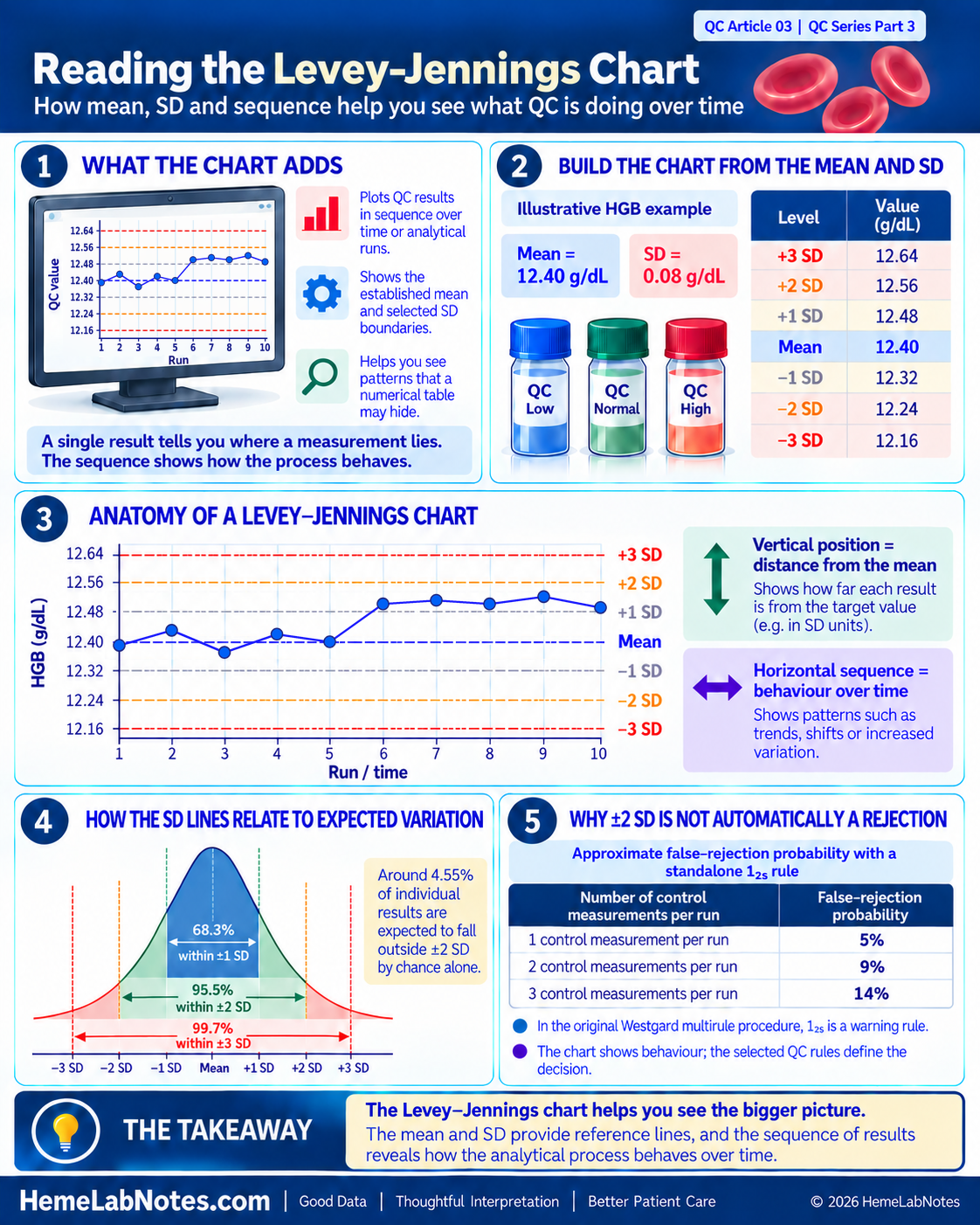
A Levey–Jennings (LJ) chart is a graphical method used to monitor quality-control measurements across successive analytical runs or time intervals.
It plots individual QC results against an established mean and standard deviation.
The chart has two main axes:
- Horizontal axis (X-axis): Time, date, analytical run or another sequential QC event.
- Vertical axis (Y-axis): The measured QC value or its corresponding SD score.
Horizontal reference lines show the established mean and selected SD boundaries, commonly including ±1 SD, ±2 SD and ±3 SD.
Each new QC result is plotted in sequence. Connecting successive measurements makes changes in the results easier to recognise.
The principle is not new. Levey and Jennings described the application of control charts in clinical laboratories in 1950, building on earlier statistical process-control methods. [1]
What does the chart add?
Imagine reviewing ten HGB control results in a numerical table.
You might notice that every value lies within its usual statistical limits.
When those same results are plotted in order, however, the first five may fluctuate around the mean while the next five remain consistently above it.
A summary mean and SD may conceal this change in sequence.
The LJ chart helps us recognise changes in the behaviour of QC measurements over time.
It shows us where a result lies and how the surrounding measurements behave. The laboratory’s established QC strategy then determines how that information should be used. [2]
2. Before Reading the Chart: Are the Mean and SD Appropriate?
A Levey–Jennings chart is only as useful as the reference values on which it is built.
Before interpreting a result above or below the mean, we must know how that mean and SD were established.
For routine laboratory QC, these values should represent an appropriately characterised measurement process, including relevant sources of variation between runs and across days.
A few consecutive measurements may provide useful initial information, but their SD mainly reflects short-term measurement conditions. It should not automatically be treated as a reliable estimate of longer-term analytical variation.
Establishing control limits
CLSI C24 discusses approaches for establishing QC target values and standard deviations and for maintaining an effective statistical QC strategy. [2]
For a new QC product, a commonly recommended approach is to collect at least 20 measurements on 20 separate days when feasible. This provides information across a broader period than a single-day repeatability study.
In practice, the laboratory may need a documented provisional approach while longer-term data are collected.
The number of observations, collection period and acceptance criteria should be appropriate to the QC material and the laboratory’s validated procedure.
The practical challenge with haematology controls
Haematology QC materials often have relatively short usable shelf lives, depending on the product and storage conditions.
This makes collecting extensive long-term data for every new control lot challenging.
One practical approach is to establish the new lot’s mean using appropriate measurements during a crossover period, while deriving the SD from the laboratory’s established long-term (cumulative) CV for the same parameter and control level.
Bio-Rad, for example, describes establishing the mean of a new lot of an existing QC product from 10 measurements on 10 different days, while carrying forward the SD or CV from the existing lot. The results should also be compared with relevant manufacturer and peer-group information when available. [3]
For example, suppose:
- New HGB control lot mean = 12.40 g/dL
- Applicable cumulative HGB CV = 0.65%
The estimated SD would be:
SD = Mean × CV (%) ÷ 100
SD = 12.40 × 0.65 ÷ 100
SD = 0.0806 g/dL ≈ 0.08 g/dL
This approach uses an established longer-term estimate of analytical imprecision rather than relying solely on the potentially small SD obtained from a short crossover study.
If an existing CV is carried forward, the corresponding absolute SD should be calculated using the new lot’s mean. Carrying forward an absolute SD and carrying forward a CV are not mathematically identical when the means differ.
The cumulative CV must also be suitable for the measurement procedure, parameter and control level. The laboratory should verify its applicability to the new material and analytical conditions before adopting final limits.
A new control lot is not the same as a new reagent lot
This distinction matters.
New control-material lot: The control material itself has changed. A new lot-specific mean must be established or appropriately verified, preferably through an overlap study with the existing lot before changeover.
New reagent lot or calibration event: The control material may remain unchanged, so a movement in its measured values is evidence requiring evaluation. It is not, by itself, a reason to reset the QC target.
Following an investigated and verified change to the measurement process, a target revision may sometimes be justified. Such a decision should follow the laboratory’s documented procedure rather than simply accommodating an unexplained shift.
For laboratories using low, normal and high haematology controls, each level also requires its appropriate reference values.
The mean establishes where the process is expected to operate. The SD describes its expected analytical variation.
Both must be suitable before the chart can be interpreted meaningfully.
3. Understanding the Lines on a Levey–Jennings Chart
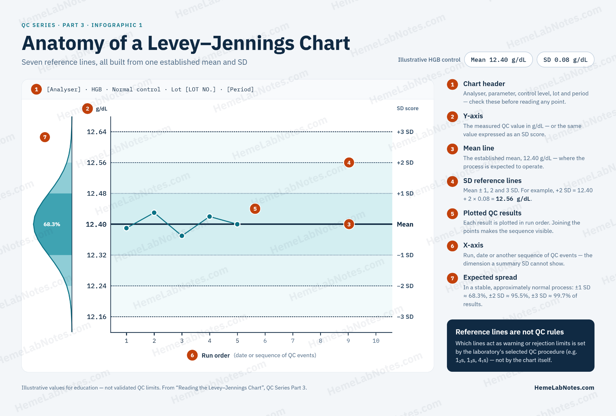
Let us continue with an illustrative HGB control.
Assume the laboratory has appropriately established:
Mean = 12.40 g/dL
SD = 0.08 g/dL
The LJ reference lines are calculated as follows.
| Chart boundary | Calculation | HGB (g/dL) |
|---|---|---|
| +3 SD | 12.40 + (3 × 0.08) | 12.64 |
| +2 SD | 12.40 + (2 × 0.08) | 12.56 |
| +1 SD | 12.40 + 0.08 | 12.48 |
| Mean | Established mean | 12.40 |
| −1 SD | 12.40 − 0.08 | 12.32 |
| −2 SD | 12.40 − (2 × 0.08) | 12.24 |
| −3 SD | 12.40 − (3 × 0.08) | 12.16 |
These values are educational examples, not universal HGB QC limits.
The step-by-step construction and interpretation of these reference lines are also described in Patricia Barry’s Levey–Jennings chart tutorial. [10]
Why are ±2 SD and ±3 SD displayed?
For a stable process whose QC results follow an approximately normal distribution:
- About 68.3% of results fall within ±1 SD.
- About 95.5% fall within ±2 SD.
- About 99.7% fall within ±3 SD.
Consequently, approximately 4.55% of individual measurements are expected to fall outside ±2 SD through ordinary statistical variation alone.
This creates an important problem when ±2 SD is used as a standalone rejection boundary.
The false-rejection problem
If every measurement outside ±2 SD causes an analytical run to be rejected, false rejections become more frequent as the number of independently evaluated control measurements increases.
| Control measurements evaluated per run | Approximate false-rejection probability with a standalone 1₂s rule |
|---|---|
| 1 | 5% |
| 2 | 9% |
| 3 | 14% |
These are the approximate instructional values reported by Westgard JO. [4]
Westgard’s figures use rounded probabilities. With an approximately 5% false-rejection probability per measurement, three independent measurements give 1 − 0.95³ ≈ 14.3%. Using the more precise normal-distribution tail probability of 4.55% instead gives approximately 8.9% for two measurements and 13.0% for three. The quoted percentages are therefore approximations rather than values all calculated from one exact underlying probability.
The calculations assume a stable process with approximately normal and independent measurements. Actual probabilities can differ when observations are correlated or when the rule is implemented differently.
For a haematology laboratory measuring three QC levels, rejecting every run because one level exceeds ±2 SD could therefore produce substantial unnecessary investigation and repeat testing.
This is one reason the original Westgard multirule procedure uses 1₂s as a warning rather than an automatic rejection rule. [5]
The ±3 SD boundary is more extreme, but the laboratory must still apply its selected QC procedure rather than treating chart lines as interchangeable rules.
4. Reading One QC Point: Where Does Today’s Result Sit?
Suppose today’s illustrative HGB QC result is:
12.53 g/dL
The established mean is 12.40 g/dL, with an SD of 0.08 g/dL.
We can express the result’s position using an SD score, also called a z-score:
SD score = (Observed result − Mean) ÷ SD
z = (12.53 − 12.40) ÷ 0.08
z = 0.13 ÷ 0.08
z = +1.625 ≈ +1.63 SD
The result appears between the +1 SD and +2 SD lines.
This tells us that the observation is approximately 1.63 standard deviations above the established mean.
But what if yesterday’s result was also above the mean?
And the day before?
One result provides a position. A sequence provides additional information about the process.
The vertical position tells us how far a measurement is from the mean. The horizontal sequence shows how measurements behave over time.
Note on reporting resolution: Values are shown to two decimal places for illustration. Many haematology analysers report HGB to 0.1 g/dL. When reporting resolution is large relative to the SD, calculated SD scores change in comparatively coarse steps. For example, with a mean of 12.40 g/dL and SD of 0.08 g/dL, successive displayed values of 12.5 and 12.6 g/dL correspond to +1.25 SD and +2.50 SD.
5. Reading the Sequence: Ten HGB QC Results
Consider ten successive illustrative measurements from the same HGB control level.
The established reference values are:
Mean = 12.40 g/dL
SD = 0.08 g/dL
| Run | HGB (g/dL) | SD score |
|---|---|---|
| 1 | 12.39 | −0.13 |
| 2 | 12.43 | +0.38 |
| 3 | 12.37 | −0.38 |
| 4 | 12.42 | +0.25 |
| 5 | 12.40 | 0.00 |
| 6 | 12.50 | +1.25 |
| 7 | 12.51 | +1.38 |
| 8 | 12.50 | +1.25 |
| 9 | 12.52 | +1.50 |
| 10 | 12.49 | +1.13 |
These are simulated educational values shown at two-decimal precision, not output from a specified haematology analyser.
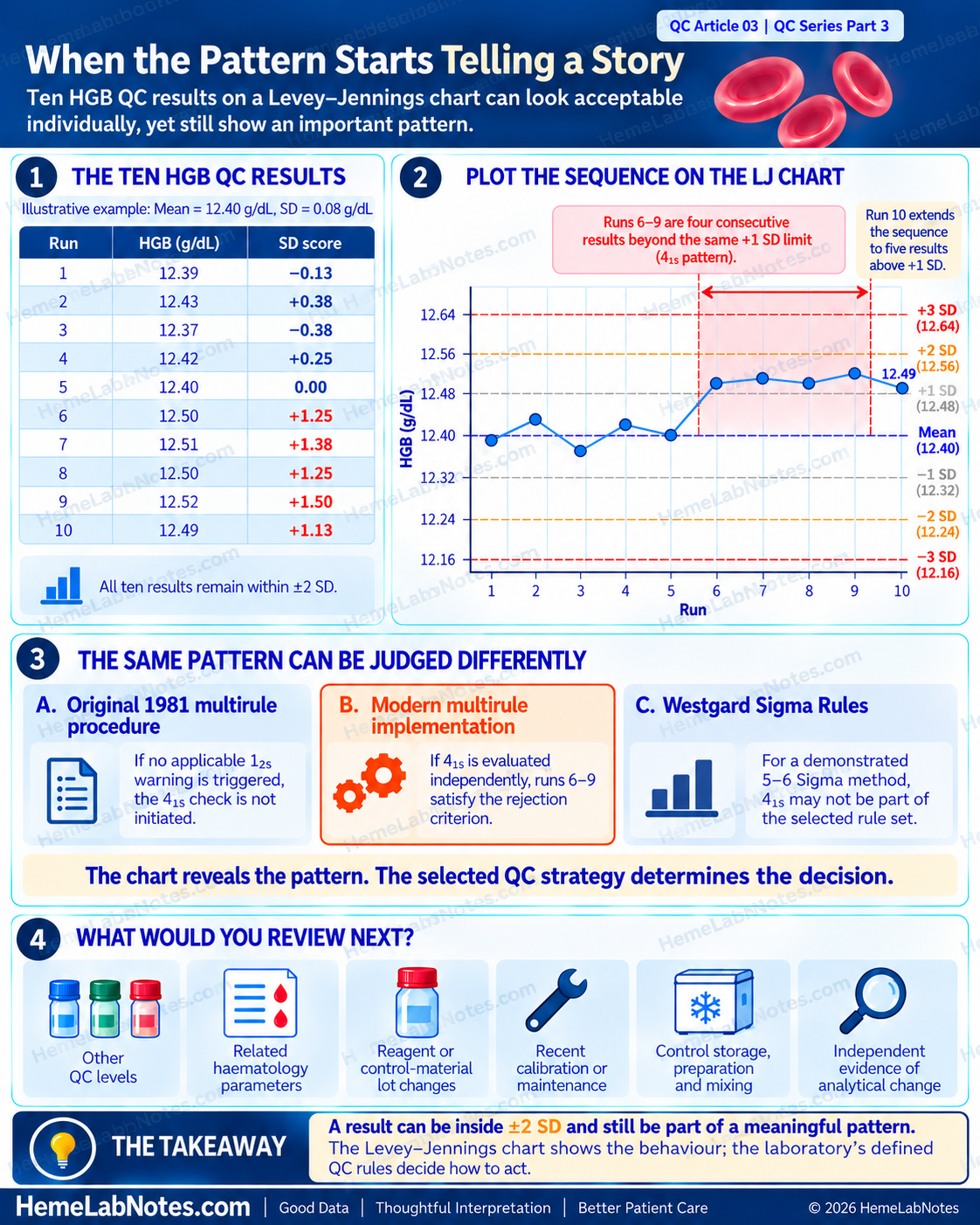
All ten measurements remain within ±2 SD.
However, their sequence reveals something important.
Runs 1–5: Fluctuating around the mean
The first five results occur above, below and directly on the established mean.
Their pattern is consistent with ordinary variation around the target, although five results alone are insufficient to establish long-term stability.
Runs 6–10: A sustained upward pattern
The following five measurements all lie above the +1 SD boundary of 12.48 g/dL.
Instead of fluctuating around the mean, the results remain consistently elevated.
This looks like a shift in the location of the QC measurements.
More importantly, the sequence raises a specific statistical QC question.
Does this sequence trigger the 4₁s rule?
Yes — it satisfies the numerical pattern described by 4₁s.
Runs 6–9 are four consecutive measurements beyond the same +1 SD boundary. Run 10 extends the sequence to five consecutive measurements.
The rejection decision depends on how the laboratory has implemented its QC rules.
Approach 1 — Original Westgard multirule procedure (1981)
The original procedure requires a 1₂s warning before the associated rejection rules are evaluated.
Because none of these ten results exceeds ±2 SD — and assuming no other control level in these runs triggered a 1₂s warning — the 4₁s check would not be initiated under the original procedure.
If another control level triggered the warning, the applicable rejection rules would need to be evaluated using the measurements and sequence defined by the laboratory’s QC procedure.
Approach 2 — Modern multirule implementation
Some modern implementations evaluate 4₁s independently, without requiring a preceding 1₂s warning.
Under an approved procedure using this approach, Runs 6–9 would satisfy the 4₁s rejection criterion.
The sequence would therefore be rejected under that rule implementation.
Approach 3 — Westgard Sigma Rules
Westgard Sigma Rules add another consideration: the analytical Sigma performance of the measurement method.
As explained by Sten Westgard, the 4₁s rule is applied in this framework when method performance is 4 Sigma or lower.
For a method demonstrated to perform at 5–6 Sigma, 4₁s is not part of the recommended rule set, so this sequence alone would not lead to rejection. [6]
This does not mean that every modern HGB method is automatically high Sigma. Sigma performance must be determined from the laboratory’s analytical performance and chosen allowable-error specification.
Three approaches, one sequence
| QC strategy | Interpretation of Runs 6–10 |
|---|---|
| Original 1981 multirule procedure, with no 1₂s warning from any applicable control | 4₁s evaluation not initiated |
| Modern multirule procedure evaluating 4₁s independently | 4₁s rejection criterion satisfied |
| Westgard Sigma Rules for a demonstrated 5–6 Sigma method, using a strategy without 4₁s | No rejection on the basis of 4₁s |
These differences are explained in Sten Westgard’s discussion of classic, modern and Sigma-based rules. [6]
The same QC data can lead to different decisions depending on the analytical performance and the statistical QC strategy selected by the laboratory.
The chart identifies the pattern. The rule implementation determines the analytical decision.
What would I examine next?
Regardless of whether the selected procedure formally rejects the run, I would want to know:
- Do other QC levels show a similar change?
- Does the pattern affect related haematology parameters?
- Has a reagent or control-material lot changed?
- Was there recent calibration or maintenance?
- Were the control materials stored, prepared and mixed appropriately?
- Is there independent evidence of a change in analytical performance?
An unusual QC pattern provides a reason to examine the measurement process. The next step is to establish whether it reflects ordinary variation, an identifiable analytical event or a genuine change requiring corrective action.
6. Recognising Different QC Behaviours
An LJ chart can reveal different forms of analytical behaviour.
| Observed behaviour | Possible interpretation |
|---|---|
| Results fluctuate around the established mean without a sustained pattern | Variation consistent with a stable process |
| One result lies unusually far from the mean | A possible isolated excursion |
| Several results remain on one side of the mean | A possible shift in process location |
| Results progressively increase or decrease | A possible trend or drift |
| Results become more widely scattered | A possible increase in analytical imprecision |
These descriptions help us recognise where further investigation may be useful.
A sustained movement away from the mean and an increase in the scatter of QC results represent different statistical behaviours. The former may suggest a change in process location; the latter may suggest increased random variation.
Distinguishing these patterns can guide troubleshooting, but formal QC decisions require the laboratory’s defined criteria.
Shift, trend and drift will be discussed in greater detail in a later article.
7. Why Being Within ±2 SD Does Not Always Mean QC Has Passed
The HGB example in Section 5 illustrates why a graphical boundary and a QC decision rule must be distinguished.
A Levey–Jennings chart shows measurements and statistical reference lines.
QC rules specify which individual results or combinations of measurements require a warning or rejection.
Some commonly used rules include:
| Rule | General interpretation |
|---|---|
| 1₂s | One result beyond ±2 SD; a warning in the original Westgard multirule procedure |
| 1₃s | One result beyond ±3 SD; commonly a rejection rule, particularly sensitive to large random-error excursions |
| 2₂s | Two consecutive results beyond the same +2 SD or −2 SD boundary, within or across runs/control levels as permitted by the procedure; mainly sensitive to systematic error |
| 4₁s | Four consecutive results beyond the same +1 SD or −1 SD boundary; sensitive to systematic error, with interpretation dependent on the rule implementation |
These descriptions summarise the principles rather than prescribing a universal ruleset. [5,7]
Why does the implementation matter?
In the original Westgard multirule design, 1₂s functions as a screening warning.
Only when that warning occurs are the associated rejection rules evaluated.
Modern computerised systems may instead evaluate selected rejection rules directly, without requiring a preceding 1₂s warning.
Westgard Sigma Rules introduce a further distinction by selecting statistical QC procedures according to method performance and the quality required for the measurement. [6]
The number of control levels also matters.
For example, 2₂s may be evaluated across specified consecutive measurements of the same control level or across different control levels within an analytical run, depending on the approved procedure.
Similarly, 4₁s may involve results across runs or levels only when that interpretation is explicitly supported by the selected rule implementation.
For designs using three control materials per run — common in haematology — Westgard also describes rules such as 2of3₂s, 3₁s, 6x and 9x as potentially more suitable for that measurement grouping. Their application still depends on the defined sequence and QC strategy. We will examine these three-level rules more closely in Part 4. [7]
A laboratory using three control levels must therefore understand how its analyser or QC software defines:
- The individual analytical run.
- The order of measurements.
- The control levels included.
- The applicable time or run boundaries.
- The warning and rejection rules.
- The action required after a rule violation.
The objective is not to activate every available rule. It is to use an appropriate QC strategy that detects clinically important analytical errors while controlling unnecessary false rejections.
A chart helps us see the behaviour. The QC rules define the decision.
8. What Should We Do When the Chart Looks Unusual?
Suppose an LJ chart shows an upward pattern similar to the example above.
The most useful response is a systematic review rather than immediately changing the target mean or repeatedly testing the same QC material until a passing value appears.
First: Confirm the data and reference limits
Check the analyser, parameter, control level, material lot, monitoring period and assigned mean and SD.
Confirm that the results belong to the correct control-material lot and have not been plotted against an unsuitable baseline.
Review whether the appearance could be influenced by the chart’s scale or display settings.
Second: Apply the documented QC strategy
Determine whether the observed sequence represents:
- A descriptive pattern requiring attention.
- A warning under the selected QC procedure.
- A formal rejection-rule violation.
The response should follow the laboratory’s established SOP and not an informal interpretation of the graph alone.
Third: Review relevant analytical events
Investigate possible changes involving reagent lots, calibration, maintenance, control preparation and storage, instrument flags and other QC measurements.
Related parameters and different control levels may help distinguish an isolated control-material issue from a broader measurement-process change.
Fourth: Resolve, document and assess patient-result impact
When an out-of-control condition is confirmed, the laboratory must investigate, perform the required corrective actions and verify satisfactory analytical performance before resuming affected patient testing or releasing results according to its procedure.
The investigation may also need to address results generated since the last acceptable QC event, including the possibility that the analytical issue began before it was detected.
ISO 15189:2022, particularly Clause 7.3.7 on ensuring the validity of examination results, supports the use of planned monitoring and appropriate internal QC procedures to identify changes in measurement performance. [8]
The WHO Laboratory Quality Management System Handbook also places QC investigation and corrective action within a broader quality-management framework. [9]
The aim is not simply to restore a green PASS indicator.
It is to restore confidence that the measurement process is producing results of the required quality.
9. Common Mistakes When Reading an LJ Chart
Mistake 1 — Looking only at today’s QC result
Today’s value may be close to the established mean, yet the preceding results may show a sustained pattern.
Reviewing the sequence adds context that an isolated measurement cannot provide.
Mistake 2 — Treating every ±2 SD excursion as an automatic rejection
A standalone 1₂s rejection rule can generate substantial false rejections, particularly when several controls are evaluated per run.
Its role must be understood within the laboratory’s selected QC procedure.
Mistake 3 — Assuming a stable chart proves analytical accuracy
A stable LJ chart provides evidence about the behaviour of the monitored control material.
It does not independently establish the absence of clinically significant bias or guarantee the accuracy of every patient result.
This limitation was discussed in QC Article 01.
Mistake 4 — Recalculating limits to accommodate an unexplained shift
Changing the QC target to follow recent results can conceal a genuine analytical change.
New control-material lots require their own appropriate targets, but an unexplained movement in an unchanged control material must be evaluated before adopting revised limits.
Mistake 5 — Confusing a visible pattern with a formally violated rule
A sequence may resemble a shift or trend without meeting a rejection criterion.
Conversely, a multi-point rule may be violated even when every individual measurement remains within ±2 SD.
The ten-run HGB example shows why both the LJ chart and the specific rule implementation are necessary.
The Takeaway
Mean and SD provide the statistical framework for quality control.
The Levey–Jennings chart adds the order of measurements, making it easier to recognise changes in analytical behaviour.
A single result tells us where a measurement lies relative to the established mean. A sequence may reveal changes in location, direction or spread.
The HGB example demonstrates something more important.
Five consecutive results above +1 SD can appear within the usual ±2 SD boundaries while satisfying the numerical pattern of 4₁s.
Whether this becomes a formal rejection depends on the selected QC strategy, including how multirule criteria are evaluated and whether the method’s Sigma performance justifies including 4₁s.
The correct interpretation therefore requires suitable control targets, appropriate SDs, a clearly defined rule set and knowledge of the measurement process.
The real value of the LJ chart is not simply drawing lines through QC measurements.
It is recognising when the measurement process deserves closer attention — and knowing how to respond before patient results are put at risk.
Coming Next — QC Series Part 4
QC Rules in Practice: When Does a Warning Become a Rejection?
Why is 1₂s sometimes treated as a warning instead of a rejection?
How do 1₃s, 2₂s and 4₁s respond to different analytical errors?
How should laboratories using three QC levels interpret rules such as 2of3₂s and 3₁s?
Why might the original Westgard multirule procedure, a modern automated implementation and a Sigma-based QC strategy reach different decisions from the same measurements?
In Part 4, we will move from reading the Levey–Jennings chart to selecting and interpreting statistical QC rules.
References
1. Levey S, Jennings ER. The use of control charts in the clinical laboratory. Am J Clin Pathol. 1950;20(11):1059–1066.
https://pubmed.ncbi.nlm.nih.gov/14783086/
2. Clinical and Laboratory Standards Institute. Statistical Quality Control for Quantitative Measurement Procedures: Principles and Definitions. 4th ed. CLSI guideline C24. Wayne, PA: CLSI; 2016.
https://clsi.org/shop/standards/c24/
3. Bio-Rad Laboratories. How to establish mean and acceptable QC ranges? QCNet Help Center.
4. Westgard JO. QC — The Chances of Rejection. Westgard QC, Basic QC Practices.
https://www.westgard.com/lessons/basic-qc-practices/lesson15full.html
5. Westgard JO, Barry PL, Hunt MR, Groth T. A multi-rule Shewhart chart for quality control in clinical chemistry. Clin Chem. 1981;27(3):493–501.
https://pubmed.ncbi.nlm.nih.gov/7471403/
6. Westgard S. 4:1s, when is it violated under different types of Westgard Rules? Westgard QC. 17 March 2026.
https://www.westgard.com/blog/4-1s-when-is-it-violated-under-different-westgard-rules.html
7. Westgard QC. Westgard Rules and Multirule Quality Control.
https://www.westgard.com/westgard-rules
8. International Organization for Standardization. ISO 15189:2022 — Medical laboratories: Requirements for quality and competence. Clause 7.3.7.
https://www.iso.org/standard/15189
9. World Health Organization. Laboratory Quality Management System: Handbook. Geneva: WHO; 2011.
https://www.who.int/publications/i/item/9789241548274
10. Barry PL. QC: The Levey–Jennings Control Chart. Westgard QC, Basic QC Practices.
https://www.westgard.com/lessons/basic-qc-practices/lesson12.html
HemeLabNotes provides practical educational material for laboratory professionals. The illustrative QC measurements and charts in this article are intended for learning and do not establish validated control limits or acceptance criteria. QC decisions and patient-result reporting must follow the laboratory’s validated procedures, applicable standards and clinical requirements.