The morning QC has passed.
All three control levels meet the laboratory’s acceptance criteria, and the analyser is ready for routine testing.
But something about the Levey–Jennings chart looks different.
Over the past few weeks, the MCV control has gradually moved upward. The individual results remain within the selected rejection limits, and the QC software has not rejected the run.
Should we investigate? Is the analyser drifting? Or is the control material itself changing?
The answer cannot be found from the shape of the chart alone.
Before deciding what caused the change, we need to establish where it is occurring, whether independent evidence supports it, and whether patient results may have been affected.
1. When QC Passes but Something Looks Different
A passing QC result tells us that the analytical process has met the laboratory’s selected acceptance criteria.
It does not prove that nothing has changed.
In Part 3, we discussed how the Levey–Jennings chart helps us recognise changes in QC results over time. In Part 4, we examined how Westgard rules help determine when a run should be rejected.
Now we need to consider what happens when an unusual pattern develops without violating the laboratory’s configured rejection criteria.
For example, an MCV control may gradually move from near its established mean towards the upper control limit.
If the laboratory uses only an individual-result rejection rule such as 1₃s, a small progressive change may not immediately trigger rejection.
A laboratory using additional rules such as 4₁s, 10x, or a trend rule may detect certain sustained patterns earlier.
The distinction matters.
QC PASS means the selected acceptance criteria have been met. It does not mean every possible analytical change has been excluded.
Equally, a visually unusual pattern is not automatically a reason to reject a run.
The appropriate action depends on the configured rules, the validity of the control limits, the magnitude of the suspected change, and the available supporting evidence.
The 2024 ICSH guidance recommends Levey–Jennings charts or similar monitoring, with trend analysis or rule-based systems, at least for the clinically important parameters WBC, RBC, HGB, MCV and PLT. It also recommends complementary internal quality control methods. [1]
The important question is not simply whether a result remains inside the control limits.
It is whether the behaviour of the measurement process deserves closer examination.
2. Shift, Trend and Drift: Defining the Patterns
These terms are often used together, but they do not describe exactly the same thing.
A shift is an abrupt change from one measurement level to another.
A trend is a directional pattern developing over successive observations.
Analytical drift is a gradual change in the analytical measurement process itself.
The key distinction is that a QC chart can show a trend without proving analytical drift.
Consider three illustrative haematology examples.
Example 1 — HGB shift after an analytical event
Imagine an HGB control with an established mean of 12.0 g/dL and SD of 0.12 g/dL.
| Run | HGB (g/dL) |
|---|---|
| 1 | 12.0 |
| 2 | 11.9 |
| 3 | 12.0 |
| 4 | 12.3 |
| 5 | 12.3 |
| 6 | 12.3 |
Illustrative data; not actual laboratory QC results.
The first three results are close to the established mean.
From Run 4 onwards, the measurements move to a higher level and remain there.
This is a typical shift pattern.
The +2 SD limit is 12.24 g/dL. Therefore, Runs 4, 5 and 6 are clearly above +2 SD.
If the laboratory uses the conventional same-side 2₂s rule as a rejection criterion, Runs 4 and 5 would trigger rejection.
Run 6 is shown only to illustrate the sustained higher level. In practice, a laboratory applying the 2₂s rejection rule would begin its investigation at Run 5, rather than continue releasing affected results while collecting further illustrative points.
This example is therefore not a passing-QC scenario.
It illustrates a visually recognisable shift that also has a clear statistical consequence under the stated rule.
Now imagine that a reagent lot change, calibration adjustment, or maintenance procedure occurred between Runs 3 and 4.
The timing gives us an important investigation clue.
But it does not prove that the event caused the shift.
We would still need to examine the associated records and other analytical evidence.
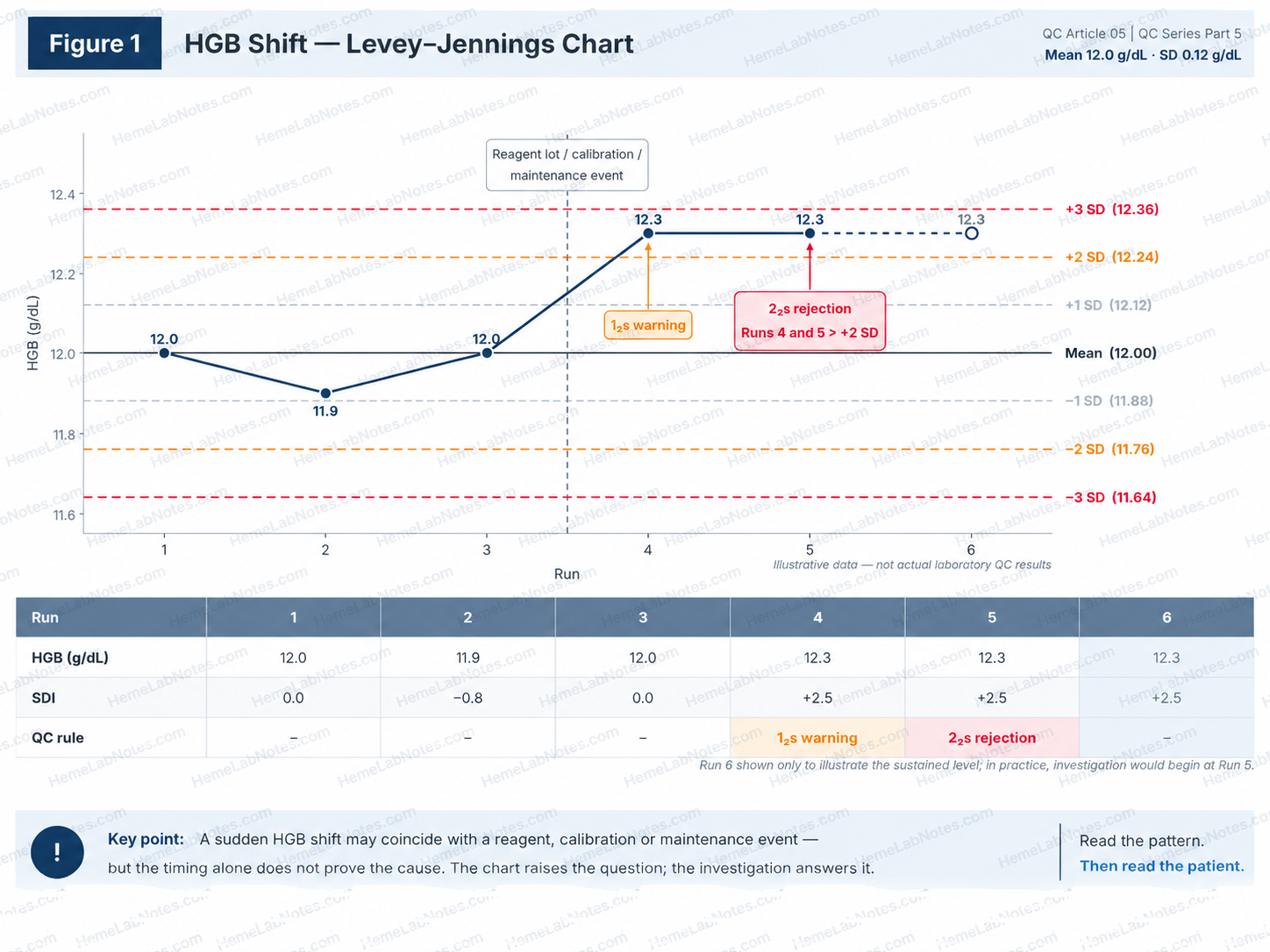
Figure 1. HGB shift: warning at Run 4 and rejection at Run 5 under the stated 2₂s rule. Run 6 is illustrative only.
View full sizeExample 2 — MCV upward trend as control material ages
Consider an MCV control with an established mean of 88.0 fL and SD of 0.6 fL.
| Day since control lot entered use | MCV (fL) |
|---|---|
| 1 | 87.9 |
| 4 | 88.1 |
| 8 | 88.0 |
| 12 | 88.3 |
| 16 | 88.5 |
| 20 | 88.4 |
| 24 | 88.8 |
| 28 | 89.0 |
Illustrative data collected across a control lot’s period of use. Individual vials must still be used within their specified open-vial stability limits.
The overall direction is upward, although the results do not increase at every observation.
The +1 SD line is 88.6 fL. Only the final two observations are above this line, and neither exceeds +2 SD.
These eight observations do not themselves form a conventional 4₁s, 7T, or 10x rejection pattern. The actual QC decision nevertheless depends on the laboratory’s configured rules and the complete QC history.
At first glance, this pattern could raise suspicion of analytical drift.
But there is another possible explanation.
Commercial haematology control materials contain stabilised cellular components. Although designed for quality monitoring, these materials can change during their usable shelf life.
Kim and colleagues investigated three commercial control systems:
- TESTPoint on the ADVIA 2120i
- e-CHECK on the XE-2100
- 6C Cell Control on the DxH 800
They observed a tendency for MCV to increase over time in all three materials. By the fifth week, most showed a deviation greater than one SD, and some exceeded four SD. [2]
This creates an important diagnostic question.
Is the analyser gradually changing, or is the control material changing while the analyser remains analytically stable for patient specimens?
A rising MCV control does not answer that question on its own.
The age of the control lot, individual vial stability, storage conditions, handling, and independent patient evidence must be considered.
When control deterioration weakens QC practice
Control-material instability may repeatedly trigger QC rules even when patient measurements have not experienced the same change.
That can create pressure to widen QC limits, repeatedly change target means, or discontinue rules that produce frequent alarms.
Westgard discussed these practical consequences in relation to the Kim study. [3]
Such responses require careful consideration.
Wider limits or less sensitive rules may reduce false rejection, but they can also reduce the probability of detecting genuine analytical errors.
A change to QC targets or rules should be scientifically justified, validated where required, documented, and approved through the laboratory’s QC policy—not made simply to make the chart look acceptable.
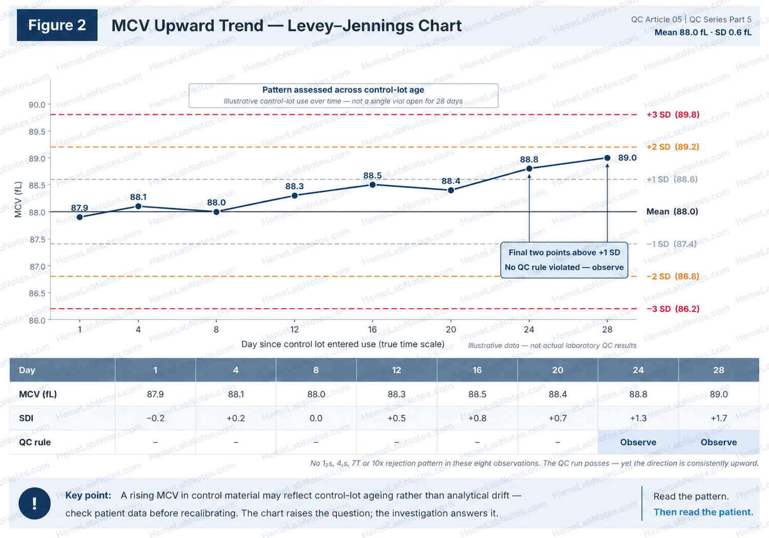
Figure 2. MCV upward trend across control-lot age. The Day 12 result is 88.3 fL; independent evidence is needed before attributing the pattern to analytical drift.
View full sizeExample 3 — PLT drift: when the analytical process may be changing
Now consider a platelet control system.
Across successive monitoring periods, all three PLT control levels gradually move upward relative to their established means.
Because the levels have different platelet concentrations and SDs, their deviations are compared using standard deviation index (SDI):
SDI = (Observed QC result − Established mean) / Established SD
The following hypothetical results show how the pattern might develop.
| QC run | L1 SDI | L2 SDI | L3 SDI |
|---|---|---|---|
| 1 | −0.3 | −0.1 | +0.2 |
| 2 | +0.2 | −0.2 | +0.1 |
| 3 | +0.4 | +0.3 | −0.1 |
| 4 | +0.6 | +0.7 | +0.8 |
| 5 | +1.1 | +1.2 | +1.3 |
| 6 | +1.4 | +1.5 | +1.3 |
Illustrative SDI values. Each level is compared against its own established mean and SD. For this example, the within-run processing sequence is L1 → L2 → L3.
The early results fluctuate around their respective means.
By Run 4, all three levels are moving in the same direction.
At Run 5, every level is beyond +1 SD.
If the laboratory applies the 4₁s rejection rule across control levels and successive runs, the three results at Run 5 followed by L1 at Run 6 constitute four consecutive measurements beyond +1 SD.
Under that configuration, the 4₁s rejection condition is met at Run 6, when the fourth qualifying measurement is obtained. Other configured pattern rules may also require action earlier.
If 4₁s is applied across levels, this later pattern may already constitute QC rejection. Even before a rejection rule is triggered, a sustained same-direction movement across all three levels deserves investigation.
Under a traditional 1₂s warning-gated multirule procedure, no result in this example exceeds ±2 SD, so the 4₁s rule would never be evaluated and the runs would pass—despite a clear same-direction movement across all three levels.
The exact rule interpretation must follow the laboratory’s approved QC configuration; laboratories should not assume every analyser or QC application evaluates measurements across levels in the same way.
This shared movement raises concern about a possible analytical change affecting platelet measurement.
But there is an important limitation.
Three QC levels from the same commercial material system are not completely independent evidence.
A common material-related effect could influence them together.
To support a conclusion of analytical drift, we would look for corroborating evidence from patient results, appropriate retained specimens, or an independent comparison process.
Until the cause is established, the most accurate description is suspected analytical drift.
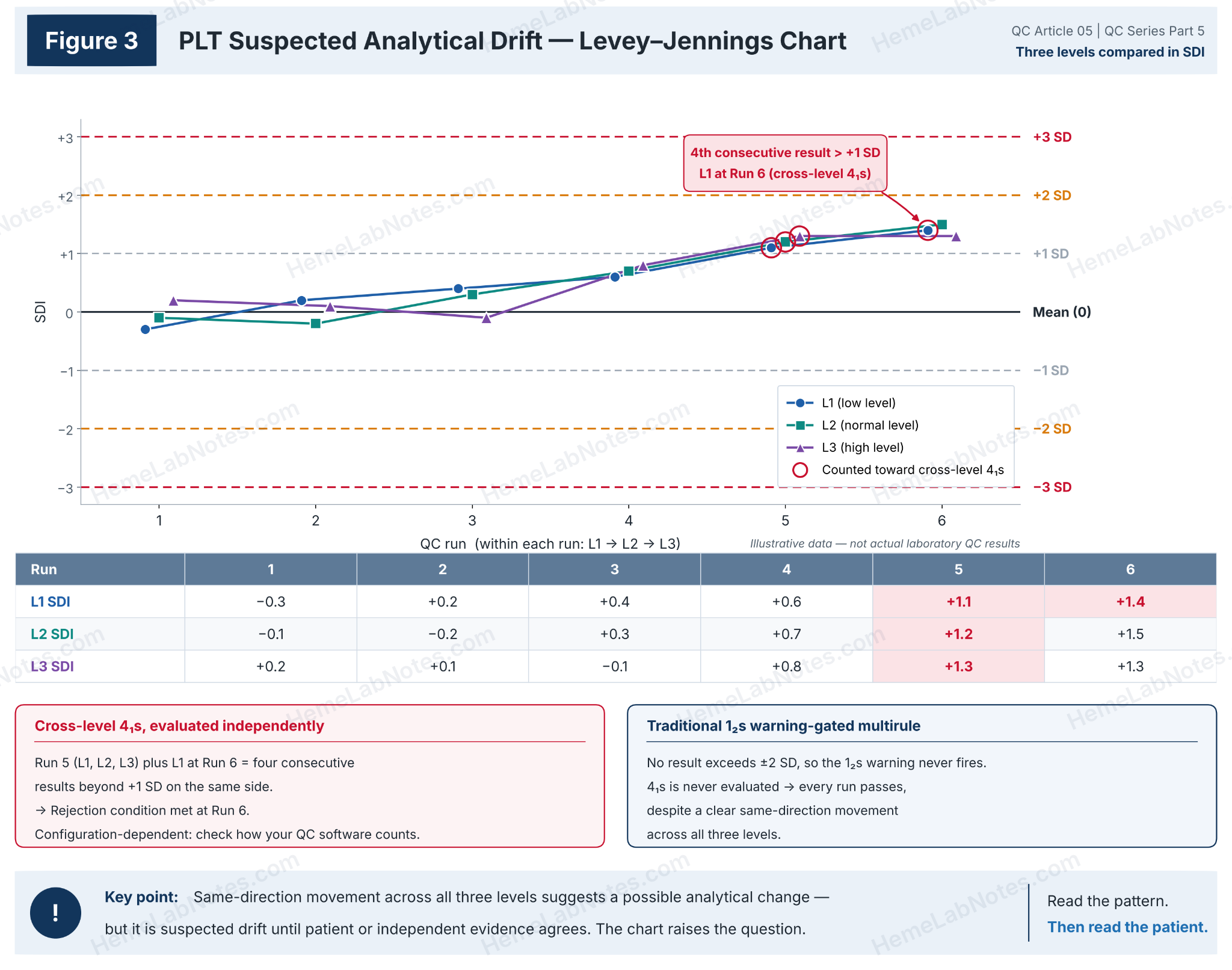
Figure 3. Suspected PLT analytical drift: cross-level 4₁s and traditional warning-gated interpretations depend on the configured procedure.
View full sizeIncreased scatter: a different kind of warning
Not every unusual QC pattern involves a change in the mean.
Suppose results remain centred near the expected mean but show a progressively wider spread.
This may suggest increased imprecision.
Possible causes include inconsistent aspiration, inadequate mixing, intermittent fluidic problems, or partial obstruction.
Those are possible investigation targets, not conclusions that can be made from the chart alone.
Shift, trend, drift and increased imprecision are therefore related quality-control concerns, but they should not be treated as interchangeable patterns.
3. Narrowing It Down: Levels, Parameters, Analysers
Once a pattern is recognised, avoid immediately blaming the reagent, calibrator, or instrument.
First, narrow down the scope of the change.
Which QC levels are affected?
Compare L1, L2 and L3.
If one level changes while the others remain stable, consider whether the finding may be related to that particular control vial, concentration range, or material behaviour.
If all three levels move together, a shared analytical factor becomes more plausible.
However, a common control-material effect remains possible.
We should also distinguish absolute differences from proportional differences.
For example, consider three PLT levels with target concentrations of 50, 250 and 500 × 10⁹/L.
A difference of +5 × 10⁹/L at every level represents approximately +10%, +2%, and +1%, respectively.
A consistent +5% shift would produce very different absolute differences.
The first pattern may suggest a concentration-independent component, while the second may suggest proportional bias.
Neither identifies the cause by itself.
Which parameters are affected?
A CBC contains related measurements, and their relationships are useful during troubleshooting.
For example, if HGB increases while RBC and HCT remain stable, both calculated MCH and MCHC will also increase.
This does not necessarily represent three independent analytical errors.
The primary change may involve HGB measurement, with the red-cell indices reflecting their calculation pathways.
The interpretation becomes even more interesting when MCV changes.
Why the analyser’s measurement pathway matters
Different haematology platforms do not derive HCT and MCV in exactly the same way.
Sysmex XN-series approach
Sysmex determines HCT from the cumulative RBC pulse information obtained during impedance measurement.
MCV is then related to the measured HCT and RBC count:
MCV (fL) = HCT (%) × 10 / RBC (10⁶/µL)
MCH and MCHC are calculated from the corresponding primary parameters.
Some Beckman Coulter platforms
On systems such as the DxH 500 series, MCV is derived from the RBC volume distribution, while HCT is calculated:
HCT (%) = RBC (10⁶/µL) × MCV (fL) / 10
The distinction is important. [4,5]
Suppose MCV increases while RBC count and HGB remain approximately stable.
On a Sysmex XN system, we should examine the underlying HCT pulse-volume measurement and its relationship to RBC.
On a system deriving HCT from MCV and RBC, an MCV change can propagate directly into the calculated HCT.
In either case, a higher HCT with stable HGB will produce a lower calculated MCHC.
The reported parameter relationships may look similar, but the underlying measurement pathways and troubleshooting priorities differ.
Understanding which parameters are measured, derived, or calculated helps us identify the likely location of a problem.
Which analyser is affected?
If the laboratory operates two haematology analysers, compare their findings.
Does the pattern occur on one analyser or both?
Did it appear after an event affecting only one instrument?
An analyser-specific change may help narrow the investigation.
But two analysers can also share reagents, calibration practices, or other common influences.
Agreement between them does not necessarily guarantee analytical correctness.
By the end of this step, the problem should be described more precisely.
Instead of:
The MCV is drifting upward.
We might say:
The MCV upward trend is present mainly in the commercial control, developed during later control-lot use, and has not yet been confirmed in patient-based monitoring.
That is a much more useful starting point for investigation.
4. Does Patient Data Tell the Same Story?
Commercial QC provides important information about analytical performance.
However, stabilised control material is not identical to fresh patient blood.
When QC begins behaving differently, patient-based monitoring can provide complementary evidence.
Patient moving averages: from Bull’s X̄B to Sysmex XbarM
Patient-based quality control has a long history in haematology.
In 1974, Bull and colleagues described methods for deriving quality-control information from patient red-cell indices using a moving-average approach designed to reduce the influence of unusual values. [6]
This became associated with Bull’s X̄B algorithm.
Modern systems have developed the approach further.
For example, Sysmex XbarM uses weighted moving-average calculations derived from Bull’s method and extends monitoring beyond the traditional red-cell indices to a broader set of CBC parameters. [7]
The principle remains useful.
Rather than relying exclusively on preserved control material, the laboratory also examines patterns derived from routine patient measurements.
Suppose commercial-control MCV gradually rises, while a properly configured patient MCV moving average remains stable.
That disagreement makes control-material instability a reasonable possibility.
But stable patient moving averages do not prove that the analyser has no analytical error.
The limitations of patient moving averages
Patient moving averages require adequate sample volume, appropriate exclusion criteria, suitable monitoring limits, and an understanding of the patient population.
Changes in the sample mix can alter the calculated average.
Examples include increased oncology specimens, changes in inpatient versus outpatient proportions, weekend activity, or the addition of a new clinical service.
Cervinski and colleagues reviewed the development, strengths and limitations of patient-based real-time quality control, including the importance of understanding patient population changes. [8]
Patient moving averages are therefore independent in terms of material, but not free from population-related influences.
Their design and detailed optimisation deserve a separate article.
Retained patient specimens
Another approach is to reanalyse suitable patient specimens within a validated stability window.
This can help assess repeatability or compare analyser performance.
ICSH Section 5.5 recommends retained fresh patient specimens less than 12 hours old as a complementary IQC method, at least daily, for imprecision assessment and inter-instrument comparison. [1]
That is a general guidance recommendation, not a guarantee of 12-hour stability for every CBC parameter.
Storage time, temperature, specimen characteristics, and analyser methodology matter.
Pintér and colleagues investigated CBC stability using the ADVIA 2120i. In samples stored at room temperature, several parameters, including MCV and MPV, showed changes after eight hours. [9]
Evidence from the Sysmex XN is also available.
Daves and colleagues studied blood samples stored at room temperature, 4°C and 37°C. [10]
At three hours, most parameters showed no meaningful bias under the evaluated conditions, apart from RDW and PLT-I at 37°C.
By six hours, meaningful bias was detected in:
- Room temperature: MCH and MCV.
- 4°C: RBC, MCHC, MCH, MCV and PLT-I.
- 37°C: RBC, RDW, MCHC, MCH and PLT-I.
In this study, refrigeration did not preserve every CBC parameter. At six hours, more of the listed parameters showed meaningful bias at 4°C than at room temperature.
The authors recommended particular caution when interpreting measurements performed more than three hours after specimen collection.
This finding is important when interpreting the ICSH recommendation concerning retained specimens less than 12 hours old.
A specimen can fall within a recommended maximum age while particular parameters have already undergone meaningful storage-related changes.
The acceptable time window for any intended comparison must therefore be based on the specific parameter, analyser, temperature, and laboratory’s validated procedure.
A stored patient specimen that has itself changed may produce a misleading indication of analyser drift.
Two-analyser comparison
A fresh patient specimen measured on two suitably verified analysers can help identify an analyser-specific difference.
But agreement between the analysers is not absolute proof of accuracy.
If both share an affected reagent lot, calibration process, or other common source of bias, they may agree while both are shifted.
The strongest conclusion comes from combining several appropriate sources of evidence, while recognising what each source cannot tell us.
5. What Could Be Causing the Change?
Only after describing the pattern and narrowing its scope should we begin evaluating possible causes.
| Possible source | Pattern that may be observed | Useful evidence |
|---|---|---|
| Control material | Level-specific change or gradual change with age | Lot history, vial age, storage records, replacement material |
| Reagent-related change | Abrupt shift or gradual change | Reagent lot changes, onboard stability, verification records |
| Calibration | Change associated with adjustment | Calibration history, factors, independent performance checks |
| Analyser performance | Persistent bias or increased imprecision | Flags, maintenance records, patient data, comparison results |
These are investigation clues, not diagnostic rules.
Control-material deterioration can produce a gradual trend.
So can a changing analytical system.
An abrupt shift may coincide with a reagent change, but coincidence alone does not establish causation.
Revisiting the MCV example
Imagine an MCV control that rises as the control lot ages.
Patient-based monitoring and suitable fresh-sample comparisons do not show a corresponding change.
This combination would support further investigation of the control material itself.
The laboratory should review the manufacturer’s stability information, the control lot’s behaviour, storage and handling records, and independent QC evidence.
Commercial-control deterioration is a possible explanation, but it must be established from evidence rather than assumed from the chart’s shape.
6. When Should We Investigate?
Not every pattern requires the same response.
The appropriate action depends on the selected QC rules, the strength of the available evidence, the potential magnitude of analytical error, and the consequences for patient results.
Three broad responses are useful.
Observe
A small deviation may justify closer observation when all selected acceptance criteria are met and no evidence suggests unacceptable analytical performance.
Observation still requires a plan.
Document the finding, review subsequent results, and identify what would trigger further investigation.
It should not mean allowing an unexplained pattern to continue indefinitely.
Investigate
Investigation becomes appropriate when a pattern persists, affects related parameters, follows a significant analytical event, or conflicts with other quality information.
Examples include an MCV trend late in the control lot’s use, an HGB shift after a reagent change, or a PLT pattern supported by patient-based monitoring.
The investigation should aim to identify the cause before selecting corrective action.
Hold affected results
Where a configured QC rejection rule has been violated, or evidence indicates potentially unacceptable analytical performance, follow the laboratory’s SOP to control affected testing and patient-result release.
Hold affected results does not automatically mean stopping every CBC result from every analyser.
The scope depends on the analytical process, parameters, derived results, and time period potentially affected.
Any continuation of testing or result release should follow the laboratory’s authorised risk-based procedures.
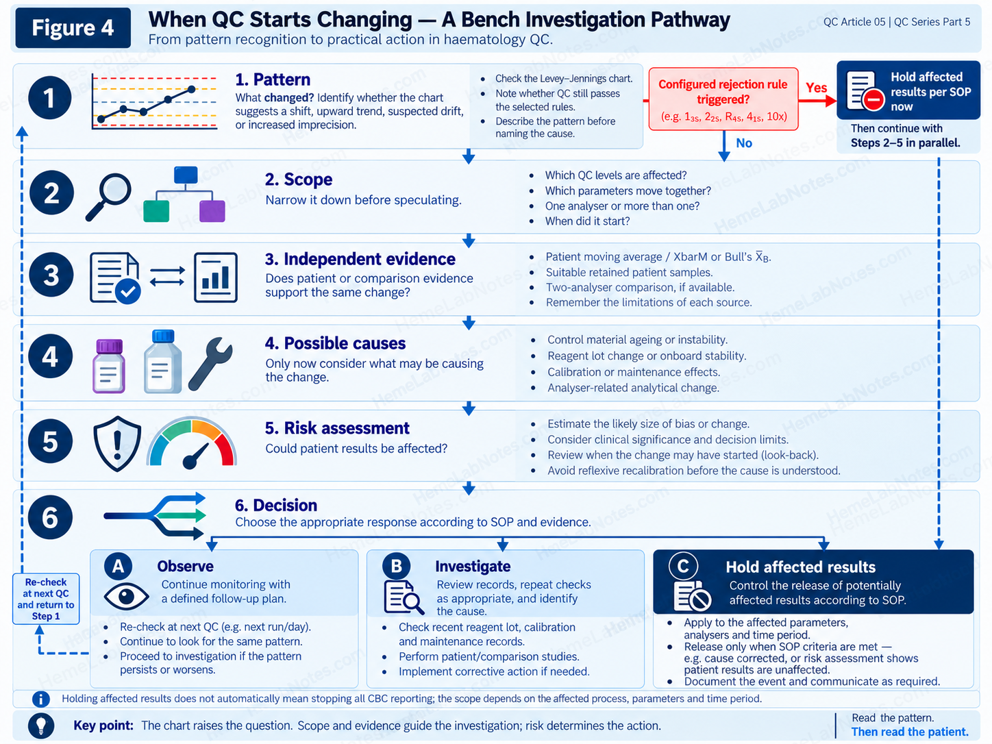
Figure 4. A bench investigation pathway, including immediate control of affected results when a configured rejection rule is triggered.
View full sizeAssess the magnitude of the possible error
When analytical bias is suspected or demonstrated, compare its magnitude with an appropriate analytical performance specification.
A relative bias may be expressed as:
Bias (%) = (Observed − Reference) / Reference × 100
The reference must be appropriate for the comparison, and the estimated difference should be interpreted in light of the reliability and uncertainty of the comparison process.
A percentage difference is not automatically clinically acceptable or unacceptable.
Analytical performance specifications may be based on clinical outcomes, biological variation, or the state of the art, depending on the measurand and intended purpose.
Sandberg and colleagues have discussed the strengths and limitations of biological-variation-based analytical performance specifications. [11]
Clinical context also matters.
An analytical shift affecting results near a clinical decision threshold may have greater consequences than a similar shift elsewhere in the measurement interval.
Determine when the change began
When patient results may have been affected, establish the potentially affected period.
Review QC history, patient monitoring trends, reagent and calibration events, analyser records, and previous evidence of acceptable performance.
Carry out the required patient-result look-back according to the laboratory’s SOP.
This may involve repeat testing, report correction, clinical notification, or documented risk assessment.
The last passing QC run may help establish a review boundary, but it does not necessarily identify the precise onset of a gradually developing error.
Avoid reflexive recalibration
An unusual QC pattern does not automatically mean recalibration is required.
If the control material is deteriorating, recalibrating the analyser to move that material back towards its original mean could introduce bias into patient measurements.
If a genuine calibration-related problem is demonstrated, corrective calibration may be necessary.
The distinction is crucial.
Recalibration should be a justified corrective action arising from the investigation—not a substitute for finding the problem.
Correcting the wrong cause may improve the appearance of the QC chart while reducing the reliability of patient results.
7. The Practical Takeaway
Shift, trend and drift are useful descriptions, but they are not interchangeable diagnoses.
A shift describes an abrupt change in measurement level.
A trend describes directional behaviour over time.
Analytical drift describes a gradual change in the measurement process itself.
Increased scatter suggests a different concern: greater measurement variability.
When the Levey–Jennings chart looks unusual, begin with the pattern.
Then narrow the scope.
Which levels are affected? Which parameters? Which analyser? Does the timing correspond to a reagent, calibration or control-material event?
Next, examine the independent evidence.
Patient moving averages, retained patient specimens and inter-analyser comparisons can help, provided their limitations are understood.
Finally, assess the potential consequences for patient results.
Three questions should remain separate:
What statistical pattern is present?
Has the analytical process actually changed?
Could the change have a clinically significant effect on patient results?
A chart cannot answer all three.
It can tell us when something deserves attention.
The investigation tells us what the evidence supports and what action is needed.
The chart raises the question; the investigation answers it.
References
-
McCafferty R, Cembrowski G, de la Salle B, Peng M, Urrechaga E. ICSH guidance for internal quality control policy for blood cell counters. Int J Lab Hematol. 2024;46(2):227–233. doi:10.1111/ijlh.14212.
-
Kim SJ, Lee EY, Song YJ, Song J. The instability of commercial control materials in quality control of mean corpuscular volume. Clin Chim Acta. 2014;434:11–15. doi:10.1016/j.cca.2014.04.004.
-
Westgard S. Pop Quiz: How Many SDIs Can a Hematology Control Drift?. Westgard QC.
-
Sysmex. The Influence of RBC Counting Technology on MCHC Results. Technical white paper. Accessed October 26, 2026.
-
Beckman Coulter. DxH 500 Series Hematology Analyzer: Technology and Case Studies. Technical documentation. Accessed October 26, 2026.
-
Bull BS, Elashoff RM, Heilbron DC, Couperus J. A study of various estimators for the derivation of quality control procedures from patient erythrocyte indices. Am J Clin Pathol. 1974;61(4):473–481. doi:10.1093/ajcp/61.4.473.
-
Sysmex Asia Pacific. Beyond Routine QC Metrics. Sysmex educational material describing XbarM and its relationship to Bull’s algorithm. Accessed October 26, 2026.
-
Cervinski MA, Bietenbeck A, Katayev A, Loh TP, van Rossum HH, Badrick T. Advances in clinical chemistry patient-based real-time quality control (PBRTQC). Adv Clin Chem. 2023;117:223–261. doi:10.1016/bs.acc.2023.08.003.
-
Pintér E, László K, Schüszler I, Konderák J. The stability of quantitative blood count parameters using the ADVIA 2120i hematology analyzer. Pract Lab Med. 2016;4:16–21. doi:10.1016/j.plabm.2015.12.001.
-
Daves M, Zagler EM, Cemin R, et al. Sample stability for complete blood cell count using the Sysmex XN haematological analyser. Blood Transfus. 2015;13(4):576–582. doi:10.2450/2015.0007-15.
-
Sandberg S, Coskun A, Carobene A, et al. Analytical performance specifications based on biological variation data – considerations, strengths and limitations. Clin Chem Lab Med. 2024;62(8):1483–1489. doi:10.1515/cclm-2024-0108.
Educational note: All numerical QC examples in this article are hypothetical and are intended for pattern recognition and laboratory reasoning. They are not actual patient results or laboratory QC data. Laboratories must follow their validated QC rules, specimen stability requirements, analytical performance specifications and documented SOPs.
HemeLabNotes
Good Data | Thoughtful Interpretation | Better Patient Care
Read the pattern. Then read the patient.